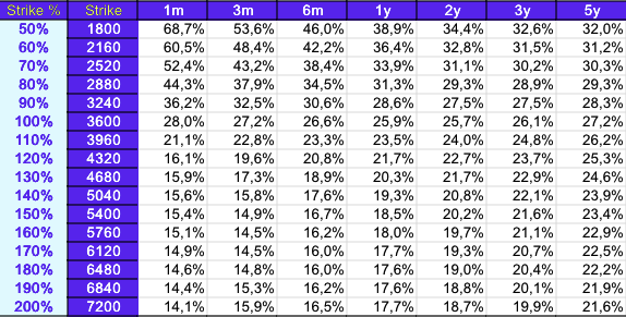
Vanilla options

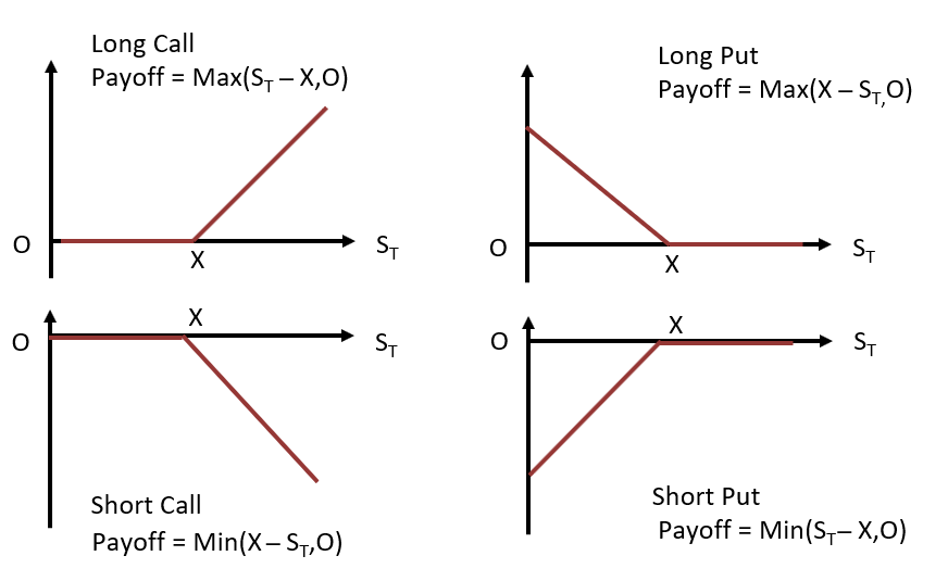
Option strategies

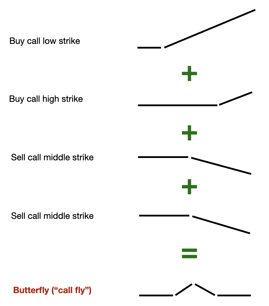
One easy way to find the payoff of a strategy that combines standard calls/puts is to decompose the payoffs.

Bull call spread

Long call with strike $K_1$ and short call with strike $K_2$ ($K_1 < K_2$). The payoff is:

\[payoff = max(K_2 - S, 0) - max(K_1 - S, 0)\]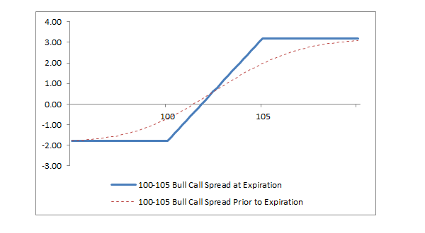

Advantages of the bull call spread:

• limited risk (the maximum loss is the net premium paid)

• lower premium than a long call (the premium paid is the difference between the two call premiums)

Call fly

Relative value volatility

This strategy is used by hedge funds. It consists in finding arbitrage looking at the volatility curves.

Example 1: look at the spread between 2 options. Say the implied volatility is steep for calls relative to puts:

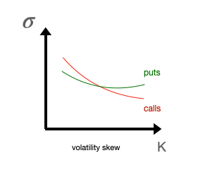
One possibility would be to sell OTM puts and buy OTM calls hoping that the spread will reduce.

Example 2: in a more sophisticated approach, one can think about looking at relationships between a pool of options.

\[spread = \alpha_0 + \alpha_1 \hat \sigma_1 + \alpha_2 \hat \sigma_2 + ...\]

The positions (long/short) would be taken based on the hope that the spread would revert to historical levels.

Electronic market-making

This strategy is used by hedge funds and rely on making a large number of trades in short times (low latency).

• volatility estimation model to know what are the “fair” implied volatilities to use for pricing -> can be B-S

• interpolation to price illiquid options -> a final volatility surface is obtained

• pricing using B-S or equivalent

• adapt bid/ask spreads depending on volatility and book risk. Example: if a lot of calls (delta positive) have been sold, the book likely has a high delta exposure, thus the HF will lower the ask of puts (delta negative) to make them more attractive and thus reduce the delta.

Note: it can be counterintuitive to use B-S twice (once to get the implied volatility, once to get the price) but it seems that this is often done like so.

Greeks

As showed in the Black-Scholes section,

\[\theta + r S \Delta + \frac{1}{2}S^2\sigma^2 \Gamma = rC\]

Delta

The delta is:

• The sensitivity w.r.t. the underlying move of 1 unit. E.g. Microsoft trades at \$410 and the ATM call is at \$4.7 with a delta of 50%. If the price moves to \$411, the call price becomes 4.7 + 0.5 = \$5.2.

• The estimated probability that the underlying ends up ITM at maturity.

• The quantity of underlying to short to be delta-hedged.

• 50% when ATM. In other words, when buying a call ATM, we earn only half of the underlying’s variation.

When a position is delta-hedged, it can still be profitable on other aspects such as theta (e.g. by selling options and collecting the time decay as time passes) or vega.

\[\Delta_{call} = \mathcal{N}(d_1)\] \[\Delta_{put} = \mathcal{N}(d_1)-1\]

$d_1 = \frac{\ln\frac{S_t}{K}+\left(r+\frac{\sigma^2}{2}\right)\left(T-t\right)}{\sigma\sqrt{T-t}}$

Gamma

The gamma is:

• The sensitivity of the delta w.r.t. the underlying move

Gamma positive: when the underlying increases a lot, the delta increases even more (so the option becomes even more sensitive to the underlying).

Example: when an investor buys a BRC, he is gamma negative (short put). It means that when the underlying decreases (and goes close to the barrier), the delta increases so the option becomes more sensitive to the underlying. Since he is also delta positive, the option would strongly decrease once close to the barrier. That’s why considering selling a structured product when the underlying arrives close to the barrier is not a good strategy.

P&L attribution

The option price is a function of the spot, the volatility and the time: $V(S, \sigma, t)$. The P&L is the price difference after a small variation of these inputs:

\[\text{P&L} = V(S + dS, \sigma + d\sigma, t + dt) - V(S, \sigma, t)\]

A Taylor expansion at the 2nd order gives:

\[\begin{aligned} \text{P&L} \approx \; & \frac{\partial V}{\partial S} dS + \frac{\partial V}{\partial \sigma} d\sigma + \frac{\partial V}{\partial t} dt \\ & + \frac{1}{2}\frac{\partial^2 V}{\partial S^2} dS^2 + \frac{1}{2}\frac{\partial^2 V}{\partial \sigma^2} d\sigma^2 + \frac{1}{2}\frac{\partial^2 V}{\partial t^2} dt^2 \\ & + \frac{\partial^2 V}{\partial S \partial \sigma} dS \, d\sigma + \frac{\partial^2 V}{\partial S \partial t} dS \, dt + \frac{\partial^2 V}{\partial \sigma \partial t} d\sigma \, dt \end{aligned}\]

Warning: the well-known formula $f(a+h) \approx \sum_n \frac{f^{(n)}(a)}{n!}h^n$ is for one variable only. With several variables, the 2nd order term is $\frac{1}{2} dx^T H dx$ (with $H$ the Hessian).

In practice, only the 2nd order w.r.t. the spot is kept. The other terms are left in the residual:

\[\text{P&L} \approx \Delta \, dS + \frac{1}{2}\Gamma \, dS^2 + \mathcal{V} \, d\sigma + \Theta \, dt + \epsilon\]

with $\epsilon$ the unexplained P&L (neglected and higher-order terms).

Note (1): this formula is not specific to Black-Scholes, it is a simple Taylor expansion of the price w.r.t. its inputs. The model (e.g. B-S) only intervenes in the computation of the greeks.

Note (2): since $dS^2 \geq 0$, the gamma contribution to the P&L is positive when gamma is positive. However, this effect can be compensated by other greeks, in particular theta (always of opposite sign).

Volatility curves

To price an option, the traders need to know the right implied volatility. Indeed, the implied volatility is the only input that is not observable in the market. In practice, the Black-Scholes model is used to find this implied volatility (rather than to compute option prices). See this tutorial for an example of a volatility curve computation.

Volatility w.r.t the strike

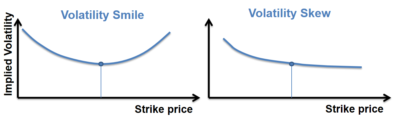
It’s the implied volatility plotted against the strike. For FX options, it has a “smile” shape. For equity options, it has a “skew” shape.

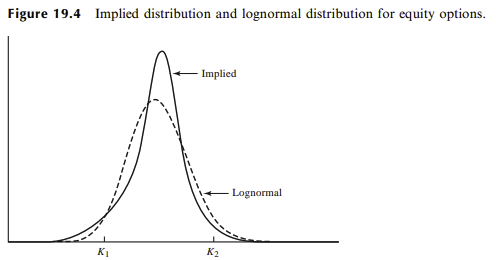
The volatility curve can be explained in computing the associated risk-neutral distribution (also called implied distribution):

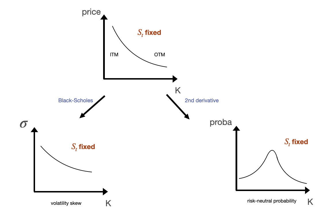
In Black-Scholes model, the assumed risk-neutral price distribution is lognormal. However, the “real” risk-neutral probability function deduced from the market option prices can look different.

For FX options, it has a larger kurtosis than a lognormal distribution. That’s because in reality, extreme events happen more often. As a result, DOTM/DITM options are more expensive (high implied volatility), hence the smile.

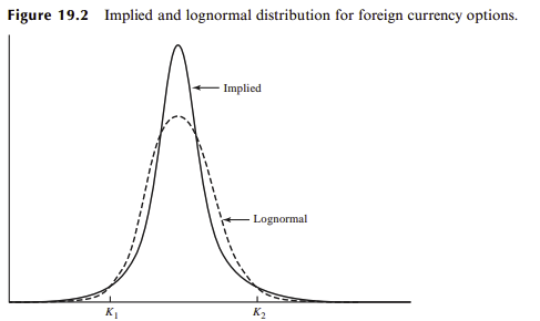
For equities options, the fat tail is mostly on the left side as investors tend to react especially strongly when the market is bearish, hence the skew. This phenomenon is less relevant in FX because FX rates typically remain stable.

Volatility term structure

It’s the implied volatility plotted against the maturity.

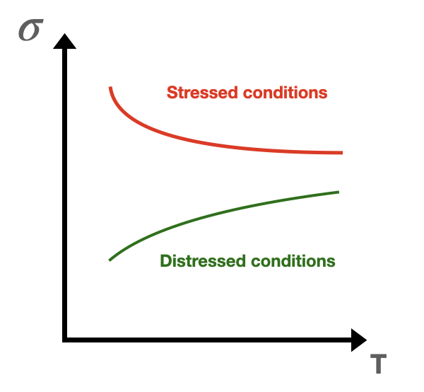
In stressed conditions, the traders are expecting a high short-term volatility.

Volatility surface

It’s the implied volatility plotted against the strike and the maturity.