Framework

Two assets:

• Risky asset (stock) with a GBM dynamics $\frac{dS_t}{S_t} = \mu dt + \sigma dW_t$

• Risk-free asset with dynamics $\frac{d\beta_t}{\beta_t} = r dt$

Warning: in previous sections, $r$ represents the risk asset returns. Here, it’s the risk-free asset.

Change of measure

A change of measure is needed to be under the risk-neutral probability and thus ensure no arbitrage opportunity. Under this risk-neutral measure, the expected return of all assets is the risk-free return.

\[\frac{dS_t}{S_t} = r dt + \sigma dW_t\]

B-S equation (largely inspired from Hull)

Let’s now consider the price of a derivative $f$. $f$ is a function of $S_t$ and $t$ and we can apply Itô’s lemma:

\[df = \Big( \frac{\partial f}{\partial t} + \frac{\partial f}{\partial S_t}\mu S_t + \frac{1}{2}\frac{\partial^2 f}{\partial S_t^2}S_t^2 \sigma^2 \Big) dt + \sigma S dB_t\]

Note (1): in the original formula, one would need to use $\mu S_t$ as drift and $\sigma S_t$ as volatility.

Note (2): the Wiener process is the same as the one driving the risky asset.

In discrete time:

\[\Delta S_t = \mu S_t \Delta t + \sigma S_t \Delta B_t \quad (*)\] \[df = \Big( \frac{\partial f}{\partial t} + \frac{\partial f}{\partial S_t}\mu S_t + \frac{1}{2}\frac{\partial^2 f}{\partial S_t^2}S_t^2 \sigma^2 \Big) \Delta t + \sigma S \Delta B_t \quad (**)\]

We can now construct a portfolio containing a stock and a derivative so that the Wiener process is eliminated.

-1: derivative (short position)

+$\frac{\partial f}{\partial S_t}$: shares

Let $V_t$ be the value of the portfolio.

\[V_t = -f + \frac{\partial f}{\partial S_t}S_t\] \[\Delta V_t = -f + \frac{\partial f}{\partial S_t}\Delta S_t\]

Using $(*)$ and $(**)$:

\[\Delta V_t = \big ( \frac{\partial f}{\partial t} + \frac{1}{2}\frac{\partial^2 f}{\partial S_t^2}S_t^2 \sigma^2 \big ) \Delta t\]

The equation doesn’t involve any Wiener process, hence the portfolio is riskless (only!) during time $\Delta t$. This implies that the portfolio must earn the same rate as the short-term risk-free asset:

\[\Delta V_t = r V_t \Delta t\]

It follows that

\[\frac{\partial f}{\partial t} + rS_t\frac{\partial f}{\partial S_t} + \frac{1}{2}\sigma^2 S_t^2 \frac{\partial^2 f}{\partial S_t^2}= rf\]

This is the Black-Scholes-Merton differential equation.

Greeks

In the case of a portfolio containing one derivative only, we define:

\[\Delta = \frac{\partial f}{\partial S_t} \quad \Gamma = \frac{\partial^2 f}{\partial S_t^2} \quad \Theta = \frac{\partial f}{\partial t} \quad\]

Hence, the BSM differential equation becomes

\[\Theta + rS_t \Delta + \frac{1}{2}\sigma^2 S_t^2\Gamma= rf\]

When the portfolio is delta-hedged ($\Delta = 0$):

\[\Theta + \frac{1}{2}\sigma^2 S_t^2\Gamma= rf\]

Call price

Under Black-Scholes, the call price is:

\[C(S_t,t) = S_t\Phi\left(d_1\right)-Ke^{-r(T-t)}\Phi\left(d_2\right)\]

with $d_1 = \frac{\ln\frac{S_t}{K}+\left(r+\frac{\sigma^2}{2}\right)\left(T-t\right)}{\sigma\sqrt{T-t}} \text{ and } d_2 = d_1 - \sigma \sqrt{T-t}$ \

We note that:

• T $\uparrow$ => price $\uparrow$ (the more the maturity increases, the more chances we have to exercise)

• K $\uparrow$ => price $\downarrow$ (the more the strike increases, the less chances we have to exercise)

• $\sigma \uparrow$ => price $\uparrow$ (the more the volatility increases, the more chances we have to exercise)

• $S_t \uparrow$ => price $\uparrow$ (the more the underlying increases, the more chances we have to exercise)

Remark: $\Phi$ is a monotonic increasing function.

Proof

We define:

\[z = \text{returns} = r_{T-t,T} = \left(r-\frac{\sigma^2}{2}\right)\left(T-t\right) + \sigma\left(W(T)-W(t)\right)\] \[z = \left(r-\frac{\sigma^2}{2}\right)\left(T-t\right) + \sigma\sqrt{T-t}\epsilon,\,\,\epsilon \sim N(0,1)\] \[z \sim N\left(\left(r-\frac{\sigma^2}{2}\right)\left(T-t\right),\sigma^2\left(T-t\right)\right)\]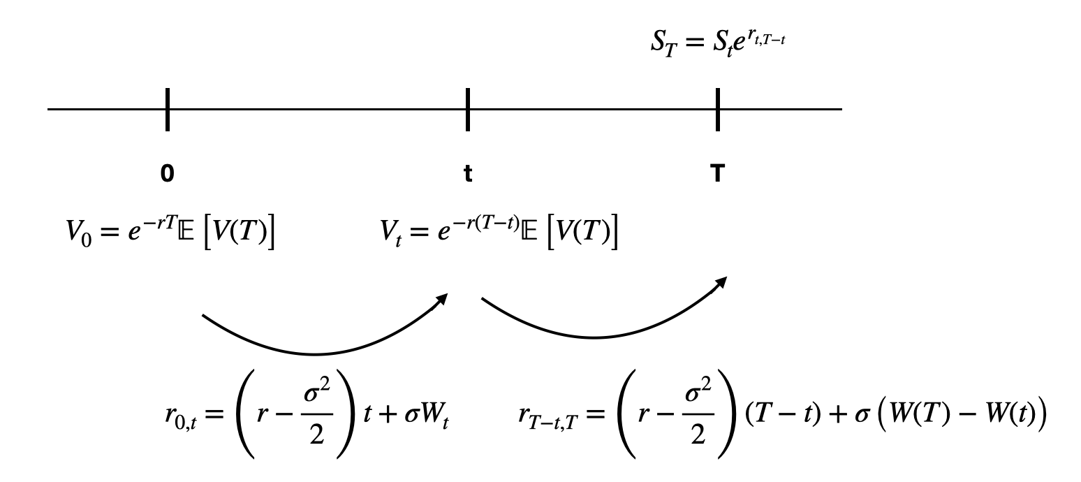

\[\begin{align*} C(S_t, t) & = e^{-r(T-t)}E^Q[f\left(S(T)\right)] ~ \text{ with } f \text{ the payoff function}\\ \,\, & = e^{-r(T-t)} \int^{+\infty}_{-\infty} f\left(S(T)\right)f(z)\,dz \\ \,\; & = e^{-r(T-t)} \int^{+\infty}_{-\infty} f\left(S_te^z\right)f(z)\,dz \end{align*}\]

The payoff of a European option is: $f(x) = \max (S_T-K,0)$

Using the fact that $S_te^z-K \leq 0$ => $z \leq \ln \frac{K}{S_t}$ and $\int^c_a f(x)dx = \int^b_a f(x)dx + \int^c_b f(x)dx$, we have:

\[\begin{align*} C(S_t,t) & = e^{-r(T-t)}\int^{+\infty}_{-\infty} \max\left(S_te^z-K,0\right)f(z)\,dz \\ \,\, & = e^{-r(T-t)}\left(\int^{\ln \frac{K}{S_t}}_{-\infty} 0\cdot f(z)\,dz + \int^{+\infty}_{\ln\frac{K}{s}} \left(S_te^z-K\right)\,f(z)\,dz\right) \\ \,\, & = e^{-r(T-t)}\int^{+\infty}_{\ln\frac{K}{S_t}}\left(S_te^z-K\right)\,f(z)\,dz \\ \,\, & = e^{-r(T-t)} \left(S_t\int^{+\infty}_{\ln\frac{K}{S_t}} e^zf(z)\,dz -K\int^{+\infty}_{\ln\frac{K}{S_t}}f(z)\,dz \right) \end{align*}\]

Reminders:

• $X \sim \mathcal{N}\left( \mu, \sigma^2 \right)$ => $f(x) = \frac{1}{\sqrt{2\pi\sigma}} e^{-\frac{1}{2}\left(\frac{x-\mu}{\sigma}\right)^2}$

• $X$ standardized => $P(X \leq x) = CDF = \int_{-\infty}^{\color{red}x} f(x)dx = \Phi\left(\frac{x-\mu}{\sigma}\right)$

• $\int_a^bf(x)dx = - \int_b^af(x)dx$

\[\begin{align*} C(S_t,t) & = e^{-r(T-t)} \left(S_t\int^{\infty}_{\ln\frac{K}{S_t}} e^zf(z)\,dz -K\int^{+\infty}_{\ln\frac{K}{S_t}}f(z)\,dz \right) \\ \,\, & = \frac{e^{-r(T-t)}}{\sqrt{2\pi}} \left(S_t\int^{+\infty}_{\ln\frac{K}{S_t}} e^{\left(r-\frac{\sigma^2}{2}\right)\left(T-t\right) + \sigma\sqrt{T-t}y}e^{-\frac{y^2}{2}}\,dy -K\int^{+\infty}_{\ln\frac{K}{s}}e^{-\frac{z^2}{2}}\,dz \right) \\ \,\, & = \frac{e^{-r(T-t)}}{\sqrt{2\pi}} \left(S_t\int^{+\infty}_{\ln\frac{K}{S_t}} e^{\left(r-\frac{\sigma^2}{2}\right)\left(T-t\right) + \sigma\sqrt{T-t}y-\frac{y^2}{2}}\,dy\right) -Ke^{-r(T-t)}\Phi\left(-\frac{\ln\frac{K}{s}- \left(r-\frac{\sigma^2}{2}\right)\left(T-t\right)}{\sigma\sqrt{T-t}}\right) \end{align*}\]

Let $A = Ke^{-r(T-t)}\Phi\left(-\frac{\ln\frac{K}{s}- \left(r-\frac{\sigma^2}{2}\right)\left(T-t\right)}{\sigma\sqrt{T-t}}\right)$

\[\begin{align*} C(S_t,t) & = \frac{e^{-r(T-t)}}{\sqrt{2\pi}} e^{\left(r-\frac{\sigma^2}{2}\right)\left(T-t\right)}\left(S_t\int^{+\infty}_{\ln\frac{K}{S_t}} e^{\sigma\sqrt{T-t}y-\frac{y^2}{2}}\,dy\right) - A \\ \,\, & = \frac{e^{-\frac{\sigma^2}{2}\left(T-t\right)}}{\sqrt{2\pi}} \left(S_t\int^{+\infty}_{\ln\frac{K}{S_t}} e^{-\frac{1}{2}\left(y^2-2\sigma\sqrt{T-t} y+\sigma^2\left(T-t\right)\right)}e^{\frac{1}{2}\sigma^2\left(T-t\right)}\,dy\right)- A \\ \,\, & = \frac{e^{-\frac{\sigma^2}{2}\left(T-t\right)}}{\sqrt{2\pi}} \left(S_t\int^{+\infty}_{\ln\frac{K}{S_t}} e^{-\frac{1}{2}\left(y-\sigma\sqrt{T-t}\right)^2+\frac{1}{2}\sigma^2\left(T-t\right)}\,dz\right) - A \\ \,\, & = \frac{e^{-\frac{\sigma^2}{2}\left(T-t\right)}e^{\frac{\sigma^2}{2}\left(T-t\right)}}{\sqrt{2\pi}} \left(S_t\int^{+\infty}_{\ln\frac{K}{S_t}} e^{-\frac{1}{2}\left(y-\sigma\sqrt{T-t}\right)^2}\,dz\right) - A \\ \,\ & = \frac{1}{\sqrt{2\pi}} \left(S_t\int^{+\infty}_{\ln\frac{K}{S_t}} e^{-\frac{1}{2}\left(y-\sigma\sqrt{T-t}\right)^2}\,dz\right) - A \\ \,\, & = S_t\Phi\left(-\frac{\ln\frac{K}{S_t}-\left(r-\frac{\sigma^2}{2}\right)\left(T-t\right)}{\sigma\sqrt{T-t}}+\sigma\sqrt{T-t}\right) - A \\ \,\, & = S_t\Phi\left(\frac{\ln\frac{S_t}{K}+\left(r+\frac{\sigma^2}{2}\right)\left(T-t\right)}{\sigma\sqrt{T-t}}\right)-Ke^{-r(T-t)}\Phi\left(\frac{\ln\frac{S_t}{K}+\left(r-\frac{\sigma^2}{2}\right)\left(T-t\right)}{\sigma\sqrt{T-t}}\right) \\ \,\, & = S_t\Phi\left(d_1\right)-Ke^{-r(T-t)}\Phi\left(d_2\right) ~~~~~ \text{ with } d_1 = \frac{\ln\frac{S_t}{K}+\left(r+\frac{\sigma^2}{2}\right)\left(T-t\right)}{\sigma\sqrt{T-t}} \text{ and } d_2 = d_1 - \sigma \sqrt{T-t} \end{align*}\]

Implementation

The above prints $2.91$. Intuitively, it means that “on average” we earn $2.91$.

With the following parameters:

$S_0 = 100$

$r = 5\%$

$K = 105$

$\sigma = 0\%$

$T = 2$

It would mean that in 2 years, the stock is certain to end at 110.25 so we would earn 5.25 exercising the option (a bit less taking the cost of opportunity into account). Now in order for NFL to hold, price $\approx$ 5 (B-S gives 4.99).

ATM price approximation

When the option is ATM, $K=S_t$, thus $d1 = \frac{1}{2}\sigma \sqrt{T}$ and $d2 = -\frac{1}{2}\sigma \sqrt{T}$. Hence the price becomes

\[C(S_t,t) = S_t \Big( \Phi\left(\frac{1}{2}\sigma \sqrt{T} \right)-\Phi\left(-\frac{1}{2}\sigma \sqrt{T}\right) \Big )\]

Using Taylor series for the first order, when $x \to 0$, $\Phi(x) \approx \Phi(0) + \Phi’(0)x$.

Reminder: Taylor series when $x \to a$, $f(x) = f(a) + f’(a)(x-a) + \frac{1}{2!}f’‘(a)(x-a)^2 + \frac{1}{3!}f^{(3)}(a)(x-a)^3 + …$

Thus $\Phi(x) + \Phi(-x) = 2\Phi’(0)x = \frac{1}{\sqrt{2 \pi }}x$

Finally, when ATM,

\[C(S_t,t) = \frac{1}{\sqrt{2 \pi }}S_t \sigma \sqrt T\]

Note: for quick calculations, $\sqrt{2 \pi} \approx 2.5$.

Note (2): this equation can be especially useful to compute the implied volatility. One could then compare the historical and implied volatility to know whether the volatility is overvalued or not. If the volatility is overvalued (implied volatility » historical volatility), premiums could be too high.