Correlation is a measure of a relationship (not necessarily linear) between two datasets.

Pearson coefficient

The Pearson correlation is a measure of linear correlation between two datasets.

$\rho_{X,Y} = \frac{cov(X,Y)}{\sigma_X \sigma_Y}$

np.cov(a,b) gives a matrix with covariances and unbiased variances (on the diagonal).

Several computation equivalences are shown below:

a = pd.Series([5, 2, 6])
b = pd.Series([18, 2, 5])

print(a.corr(b) # biased standard deviation estimators !!
          == np.corrcoef(a,b)[0,1] 
          == (np.cov(a,b)[0,1] / np.sqrt(np.cov(a,b)[0,0]*np.cov(a,b)[1,1]))
          == np.cov(a,b)[0,1] / (np.std(a,ddof=1)*np.std(b,ddof=1)) 
          != np.cov(a,b)[0,1] / (np.std(a)*np.std(b)))

# prints True

Note: when we compute those statistics numerically, we use empirical values.

Thus, $\mathbb{V}[X] = \mathbb{E}[X-\mathbb{E}[X]]$ is computed as $var_n(x)=\frac{1}{n}\Sigma(x_i - \overline{x})^2$

In the below graph, the two samples are highly correlated (pearson = 98%).

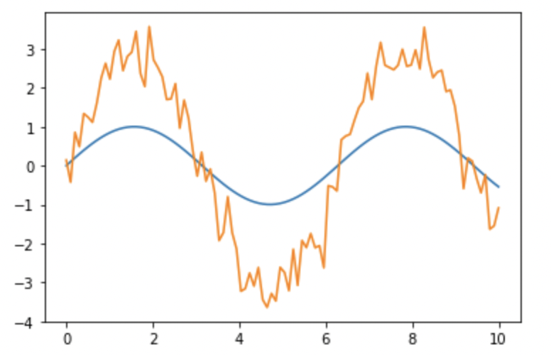
The linear trend appears when plotting one sample against the other.

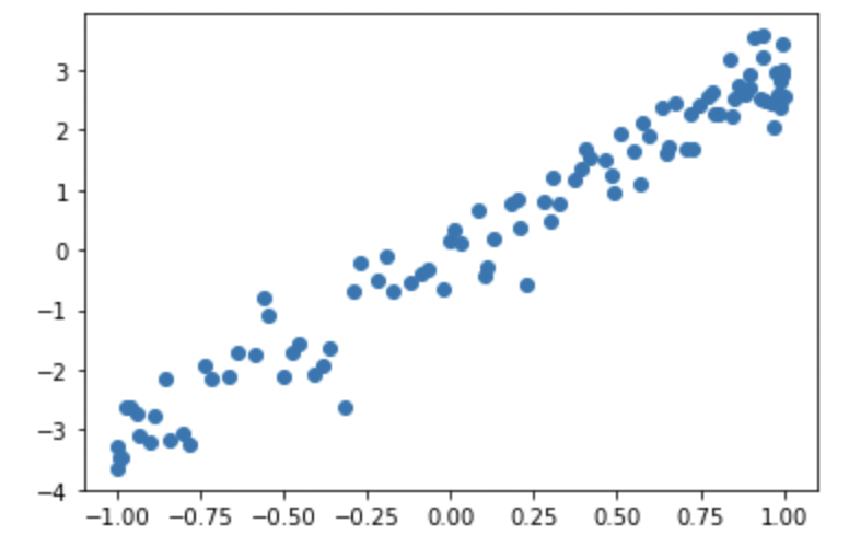
Warning: the Pearson coefficient is NOT sensitive to the scale (see relationship metrics).

Autocorrelation

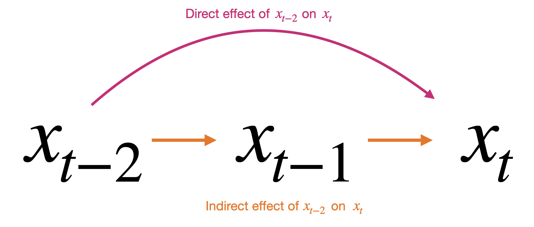
Say we want to find the correlation between returns at time $t$ and returns at time $t-2$. We could estimate $\beta_1$ in a univariate regression:

In doing so, we are effectively looking for autocorrelation. Autocorrelation considers 2 effects:

• Direct effect: $x_{t-2}$ on $x_t$

• Indirect effect: $x_{t-2}$ on $x_t$ through $x_{t-1}$ (i.e. $x_{t-2}$ on $x_{t-1}$ and then $x_{t-1}$ on $x_t$)

The autocorrelation can also be estimated using the classical Pearson correlation formula $\frac{cov}{\sigma \sigma}$. Depending on the implementation, there can be slight differences on the series used to compute each term (see formula 1 and 2).

Note that the 2 approaches (regression coefficient vs Pearson coefficient) are equivalent. Indeed, if the data are standardized and if there is only one independent variable, the correlation is equal to the regression coefficient $\beta_1$ (see relationship metrics).

Formula (1)

$R_{k} = \frac{\mathbb{E}[(X_i-\mu_X)(X_{i+k}-\mu_X)]}{\sigma_X^2}$

$X_i$ is the dataset without the last $k$ values

$X_{i+k}$ is the dataset without the first $k$ values

$\mu_X$ is the mean on the whole dataset $X$

$\sigma_X^2$ is the variance on the whole dataset $X$

Formula (2)

$R_{k} = \frac{\mathbb{E}[(X_i-\mu_{X_i})(X_{i+k}-\mu_{X_{i+k}})]}{\sigma_{X_i}\sigma_{X_{i+k}}}$

$X_i$ is the dataset without the last $k$ values

$X_{i+k}$ is the dataset without the first $k$ values

$\mu_{X_i}$ is the mean on dataset $X_i$

$\sigma_{X_i}$ is the standard deviation on dataset $X_i$

statsmodels.tsa.stattools.acf uses formula (1).

np.autocorr uses formula (2).

Below is the summary of equivalences:

import statsmodels.tsa.stattools as sm

s = pd.Series([5, 2, 6, 18, 2, 5])

a = pd.Series([5, 2, 6])
b = pd.Series([18, 2, 5])

# Formula (1)
print(s.autocorr(3) # unbiased standard deviation estimators !!
          == a.corr(b)
          ==  np.cov(a,b)[0,1]/(np.std(a,ddof=1)*np.std(b,ddof=1)))

# prints True

# Formula (2)
def acf_by_hand(x, lag):
	y1 = np.array(x[:(len(x)-lag)])
	y2 = np.array(x[lag:])
	sum_product = np.sum((y1-np.mean(x))*(y2-np.mean(x)))
	return sum_product / (len(x) * np.var(x))

print(round(acf_by_hand(s,3),6)
            == round(sm.acf(s)[3],6)) # biased covariance and standard deviation estimators !!

# prints True

Below a graphical comparison of both formulas:

import statsmodels.tsa.stattools as sm

s = pd.Series([5, 2, 6, 18, 2, 5])

corr_statsmodel =  sm.acf(s)[1:4]
corr_pandas = [s.autocorr(i) for i in range(1,4)]

test_df = pd.DataFrame([corr_statsmodel, corr_pandas]).T
test_df.columns = ['Pandas Autocorr', 'Statsmodels Autocorr']
test_df.index += 1
test_df.plot(kind='bar', title='Comparison with different lags')

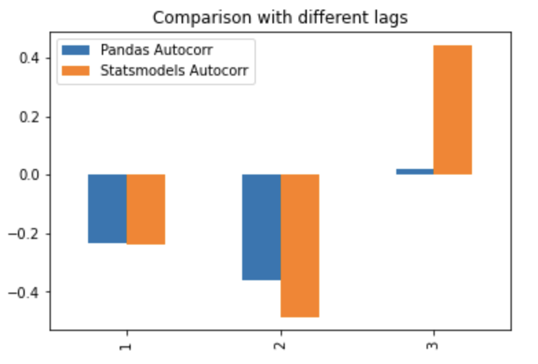
Note: the differences may get smaller for longer time series but are quite big for short ones.

Partial autocorrelation

Using the same example as above, say we want to find the correlation between prices at time $t$ and prices at time $t-2$.

This time, the model explicitly considers the direct and indirect effects. The partial autocorrelation consists in focusing on the direct effect only i.e. $\beta_2$ (=> “partial” autocorrelation).

Based on article understanding-partial-auto-correlation (towardsdatascience)

$X_t | X_{t-1} … X_{t-k+1}$ is the residual of regression $X_t = \beta_0 + \beta_1 X_{t-1} + … + \beta_k X_{t-k+1}$

$X_{t-k} | X_{t-1} … X_{t-k+1}$ is the residual of regression $X_{t-k} = \beta_0 + \beta_1 X_{t-1} + … + \beta_k X_{t-k+1}$

Thus, one can write:

$PR_k = \rho_{\epsilon_t,\epsilon_{t-k}}$

In practice, common packages such as statsmodels use methods such as Yule Walker to compute the regression coefficients and cope with the matrix inversion.

We use partial autocorrelation in order to define the order $p$ in which we can compute an AR(p) model.

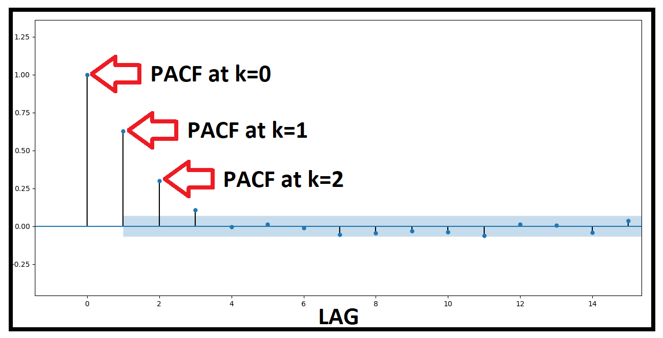
Based on this graph, we can use an AR(2) or even AR(3) ($k=3$ is just outside the 95% confidence interval.