Note: in the below example, no Monte Carlo simulation are done per se. We use only closed-form formulas.

Quantiles

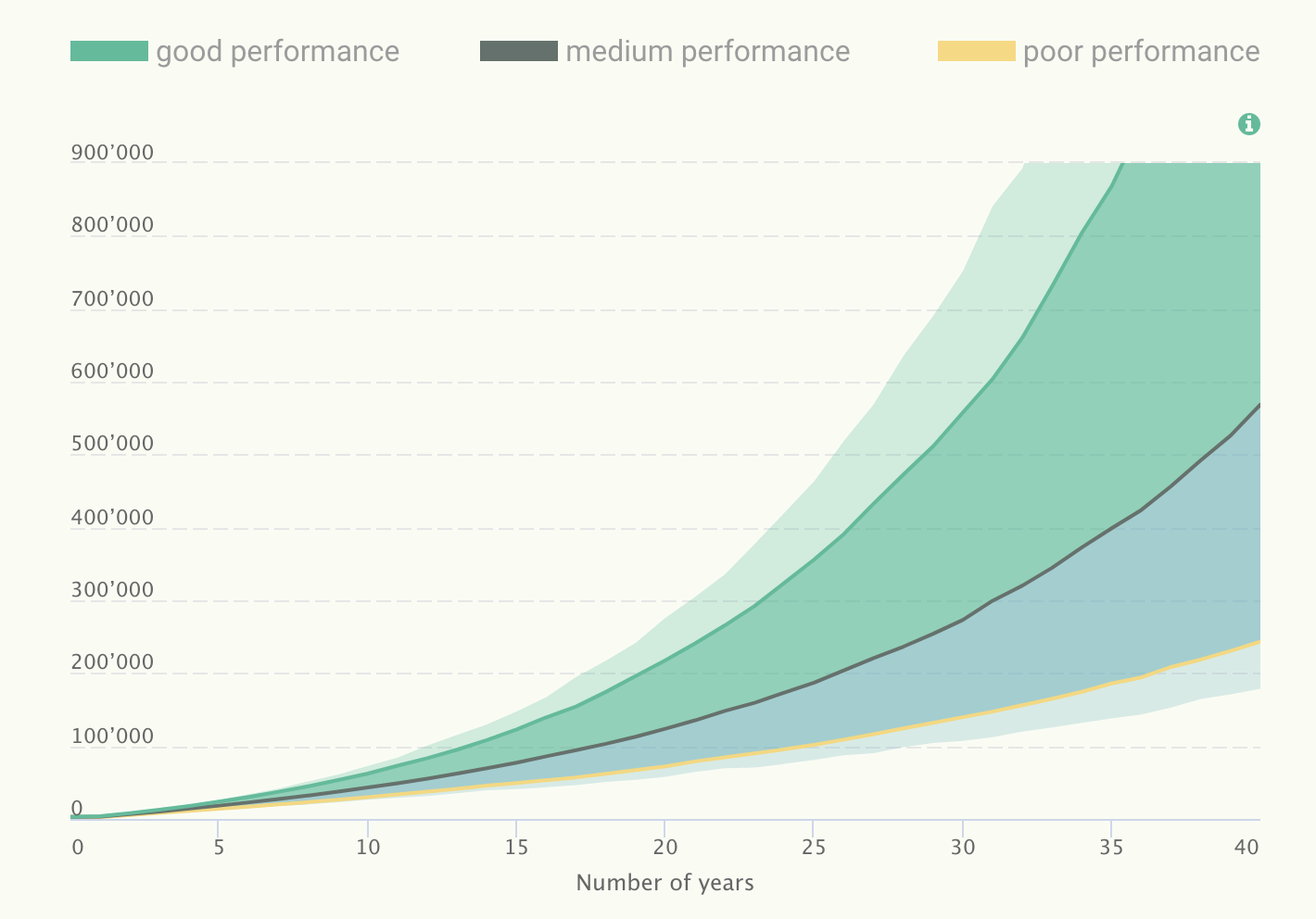
Quantiles are often showed when doing projections. They help investors assessing their risk and give a nice “trumpet” shape as showed below:

To find these upper/lower lines, at each time step we need to find quantiles of a lognormal distribution:

(i) Estimated solution

The estimated solution uses Monte Carlo simulations. It consists in taking, at each time step, quantiles associated with certain percentiles. See the implementation in the code below.

(ii) Analytical solution

To find the quantiles of a lognormal distribution, we first find quantiles of a normal distribution. We know that in the geometric Brownian motion model, returns are normally distributed:

To find the quantile of a percentile $p$, we use the quantile function:

The quantile function of a normal distribution is (source):

In scipy, the function is obtained norm.pff(p, loc=mu, scale=sigma).

# Simulations with quantiles

mu = 0.05
nYears = 10
nPeriods = 12
nPaths = 1000
sigma = 0.1
dt = 1/nPeriods
x0 = 100

St = np.zeros((nPaths, nYears*nPeriods+1))
St_exp, St_int_down_1, St_int_down_2, St_int_up_1, St_int_up_2 = \
                        [np.zeros(nYears*nPeriods+1) for i in range(5)]
St[:,0], St_exp[0], St_int_down_1[0], St_int_up_1[0], St_int_down_2[0], St_int_up_2[0] = \
                        [x0 for i in range(6)]

for t in range(1,nYears*nPeriods+1):
    St[:,t] = St[:,t-1]*np.exp((mu-(sigma**2)/2)*dt+\
    		sigma*np.random.normal(0,1,nPaths)*np.sqrt(dt))
    St_exp[t] = x0*np.exp(mu*t*dt)
    
    # estimated value (MC)
    St_int_down_1[t] = np.percentile(St[:,t],2.5)
    St_int_up_1[t] = np.percentile(St[:,t],97.5)
    # quantile function
    St_int_down_2[t] = x0*np.exp(norm.ppf
    				(
    				0.025,
    				loc=(mu-(sigma**2)/2)*(t*dt),
				scale=sigma*np.sqrt(t*dt)
				))
    St_int_up_2[t] = x0*np.exp(norm.ppf
    				(
				0.975, 
				loc=(mu-(sigma**2)/2)*(t*dt), 
				scale=sigma*np.sqrt(t*dt)
				))
    
plt.figure(figsize=(20,10))
# plt.plot(St.T, alpha=0.05)
plt.plot(St_exp, label='expected')
plt.plot(St_int_down_1, color='r')
plt.plot(St_int_up_1, label='percentiles (estimated)', color='r')
plt.plot(St_int_down_2, color='g')
plt.plot(St_int_up_2, label='percentiles (analytical)', color='g')
plt.legend()
plt.show()

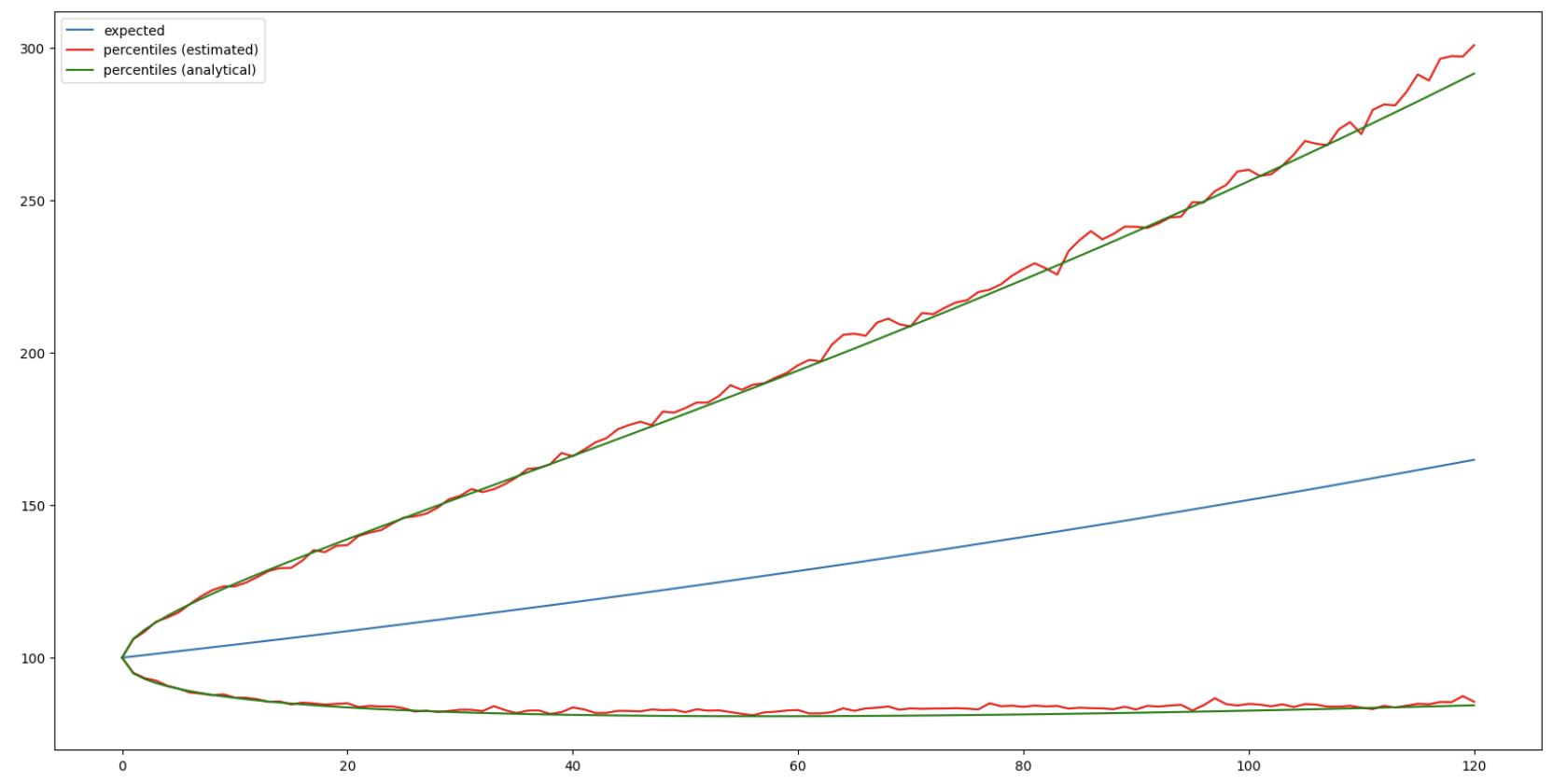
Note: such interval is often loosely called “confidence interval”. However, one can quickly see that it’s not a confidence interval because:

• it’s not built around any estimator, rather around the median (50th percentile)

• increasing the number of observations doesn’t reduce the interval

Returns

In addition to the path values, one can compute the annualized return (see discrete returns) to have an idea about the general performance in the different scenarios. This return shouldn’t be interpreted as the exact return of the path because it’s assumed to be constant over time, while in GBM the return is a random variable. In a nutshell, the annualized return answers the question: “What constant return would reproduce this final value if applied over T years?”.

Cash flows

When doing wealth planning, considering cash flows is crucial. Cash flows are associated to life events that can significantly impact the wealth.

From an implementation perspective, a cash flow is a pair [date, amount].

When doing recursive computation, the portfolio value is computed at each step. Thus, we can simply add the cash flow to the right period. The new value of the portfolio will be propagated to the next time steps and thus the cash flow amount is used in the capitalization (reminder: capitalization is the opposite of discounting).

E.g. if a cash flow happens at a date $t_0$:

Note (1): when doing monthly simulations, the cash flow amount needs to be capitalized for the remaining number of days in the month.

# Wealth projection - monthly simulations

mu = .05
n_years = 5
sigma = .1
dt = 1/2
n_periods = int(n_years/dt)
S0 = 100
n_paths = 1000

St = np.zeros((n_paths, n_periods+1))
St_exp = np.zeros(n_periods+1)
St_exp[0], St[:,0] = S0, S0

dict_CF = {
        3:20, # one cash flow = (date -> value)
        8:-10
}

for t in range(1,n_periods+1):
    CF = 0
    if t in dict_CF.keys():
        CF = dict_CF[t]
        # TODO: the cash flow amount should be capitalized 
        # for the remaining days of the month
    St[:,t] = St[:,t-1]*np.exp((mu-sigma**2/2)*dt+\
    				sigma*np.random.normal(0,1,n_paths)*np.sqrt(dt))+CF
    St_exp[t] = St_exp[t-1]*np.exp(mu*dt)+CF 
    
plt.figure()
plt.plot(St.T, alpha=.1)
plt.plot(St_exp, color='r')
plt.show()

Note (2): when considering cash flows as pairs [date, amount], we can’t distinguish between run-off and recurrent cash flows. The only way is thus to treat all cash flows as run-off cash flows. We thus don’t adjust the first cash flow of a recurrent serie.

Example: today = 10/06/2022 // recurring cash flows: 10000 every 25th => since today is the 10th, theoretically the first cash flow of the serie should be adjusted. However as mentioned above we can’t distinguish run-off cash flows from recurrent ones. Thus the first cash flow is not adjusted.

Cash flow timing

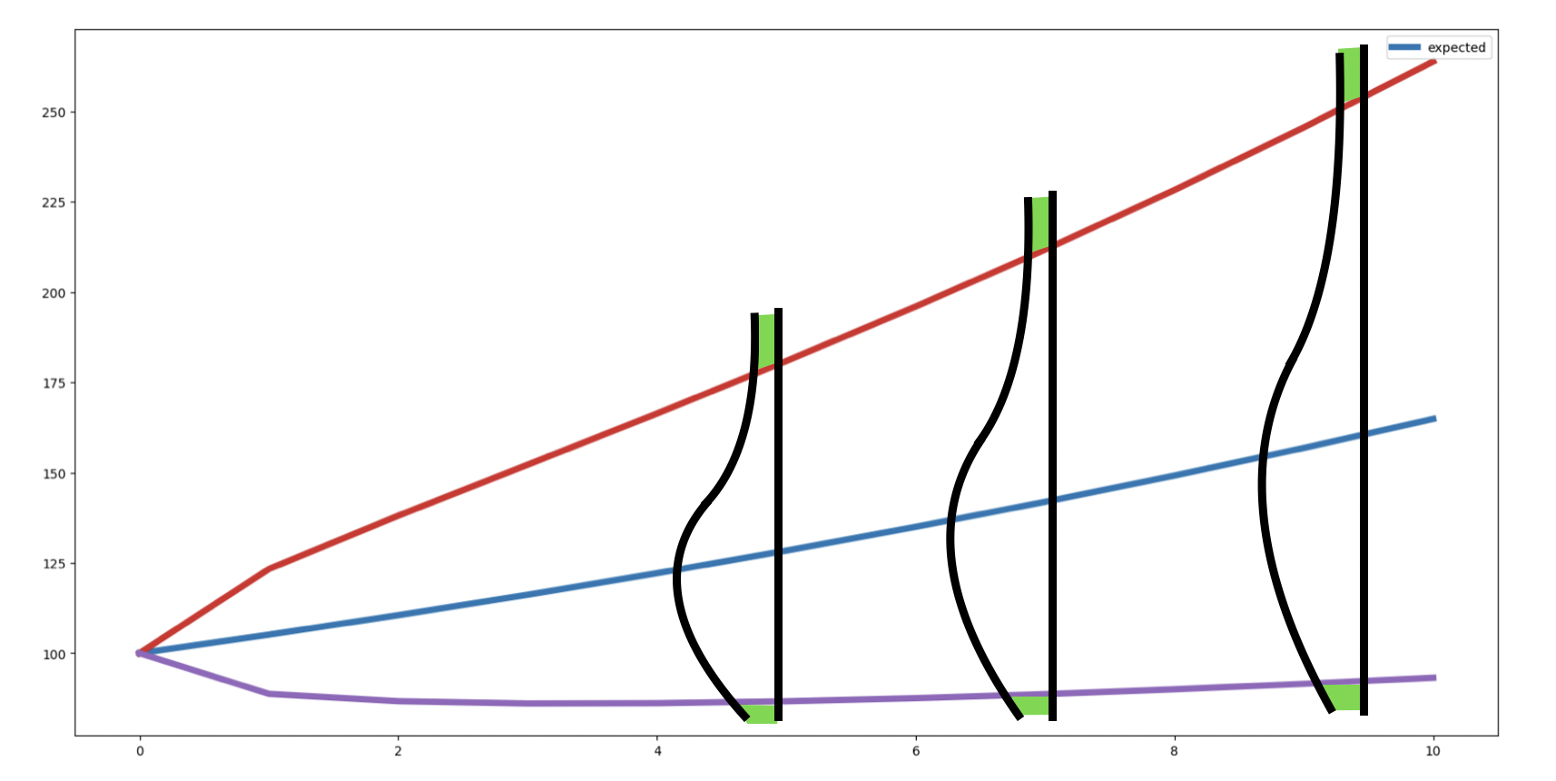
Deciding when to invest can change significantly the final return. This can be explained by the fact that the multiperiod return (also called TWR) doesn’t consider any inflow/outflow and rather only growth rates. In other words, the return is computed as if we had invested everything at the very beginning but in reality we can mitigate bad performance if we invest small amounts regularly.

We illustrate this concept with two investing approaches: lump-sum investing VS dollar-cost averaging.

Lump-sum investing: invest a large sum of money all at once.

Dollar-cost averaging: invest a fixed amount on a regular basis, regardless of the share price.

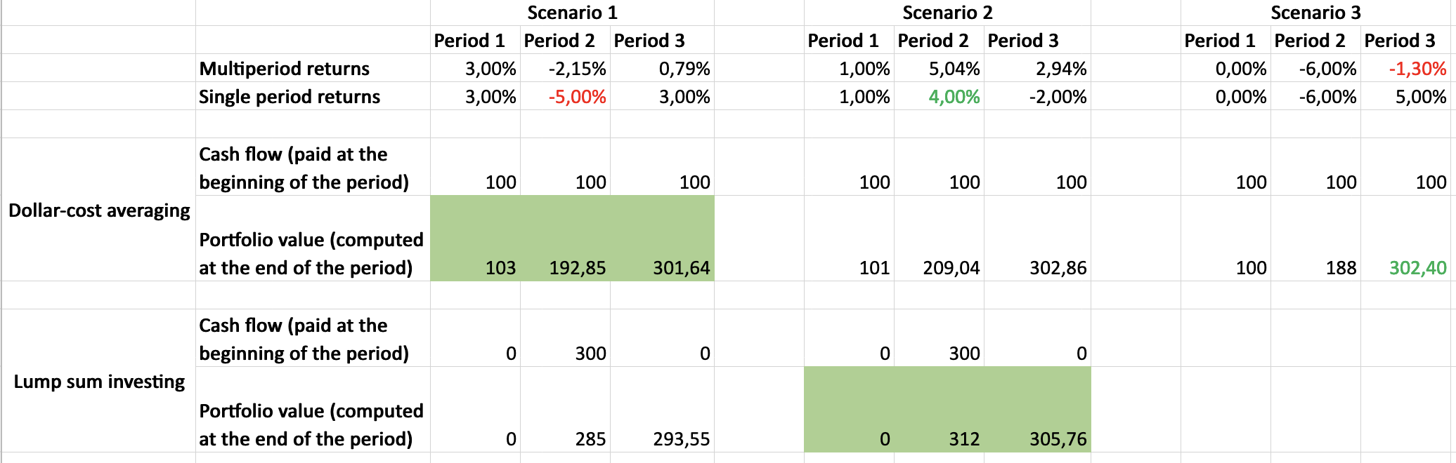
In scenario 1, more money is impacted by the negative performance => dollar-cost averaging is preferable.

In scenario 2, more money is impacted by the positive performance => lump-sum investing is preferable.

In scenario 3, we show that we can achieve gains even with a negative compounded return.

To sum up, lump-sum investing would make sense if the investor is confident that the market will go up in the coming period(s).

For risk-averse investors, dollar-cost averaging would make more sense. Indeed, since prices can move up or down, this approach somehow ensures that the paid price is the average one. In other words, this smooth out the market volatility.

In general, studies show that LSI (lump sum investing) is more profitable than DCA for long term investment. This is because markets tend to increase over time. This study did a thorough comparison over the last 30 years and gives the pros and cons.

We can also confirm such findings in a simple analysis. In the below code, we assume the investor who does LSI invest 100,000 in one initial payment. Then, we assume the investor who does DCA invests 80,000 as a first deposit and splits the rest over 6 months. The highlighted lines are the expected paths (= average of all simulations).

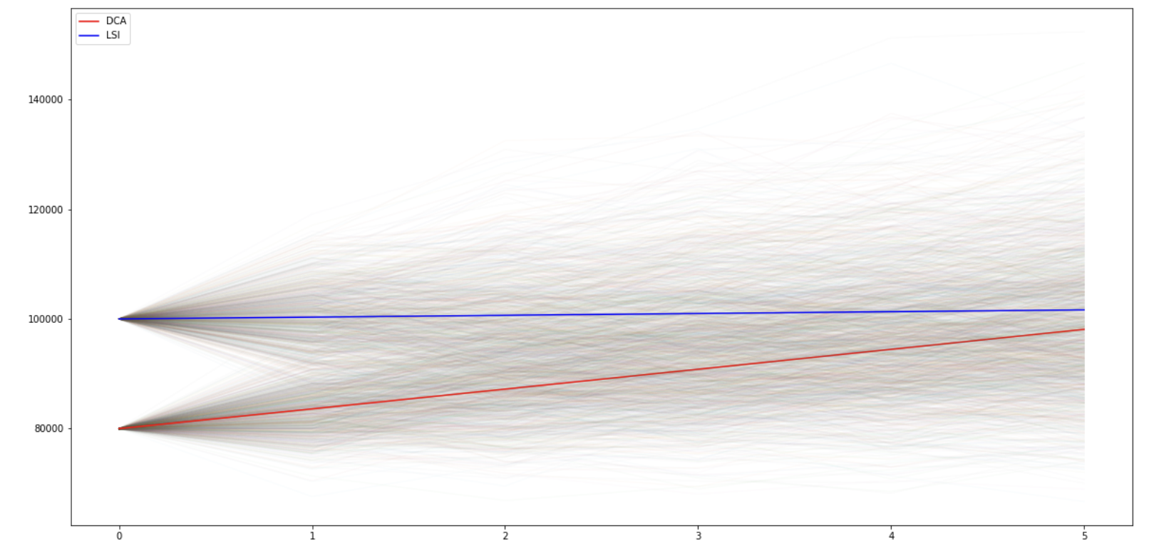
We can see that, on average, LSI outperforms DCA.

See the discrete returns section to have an overview about portfolio performance computation.

Inflation

The inflation could be considered in 2 ways:

• At portfolio level. The portfolio value is discounted by the inflation rate so that the real value is displayed.

• At cash flow level. The cash flow amount is capitalized. Example: I plan to buy a house in $x$ years. The price will certainly increase in the coming years so I will have to pay a higher amount than the today’s price => price needs to be capitalized over the years.