Discrete = payment at discrete points of time. Sometimes also called “arithmetic returns” or “linear returns” (example).

Single period returns

Single period returns are returns computed between 2 periods.

Note: the usual normality assumption is on the single period returns.

Multiperiod returns

Multiperiod returns are returns computed over several successive periods. It is based on the fact that returns are reinvested or compounded.

Example:
Let's consider a mutual fund yielding 5%/year.
No reinvestment:
\$100 in year 1 yields \$105.
\$100 in year 2 yields \$105.
Total earned = \$10.
With reinvestment:
\$100 in year 1 yields \$105.
\$105 in year 2 yields \$110,25.
Total earned = \$10,25.

When computed over $k$ periods:

Multiperiod returns can also be expressed in terms of single period returns:

$R_x$ are single period returns and $R_{x,y}$ are multiperiod returns or time weighted return (TWR) for portfolio return (see below).

It can also be called “cumulative returns”. Indeed, we notice the cumulative product:

returns = np.random.normal(0, 0.05, (4)) # single period returns are normally distributed
cumul_returns = (1+returns).cumprod()-1 # last value is the total return over the 4 periods
initial_val = 100
final_val = initial_val*(1+returns[0])*(1+returns[1])*(1+returns[2])*(1+returns[3])
final_val/initial_val-1 == cumul_returns[-1] # returns True

If we assume a fixed return rate:

Let $A$ be the value at the end of the $k$ periods and $P$ (principal) be the initial invested amount, we end up with the famous compounding equation:

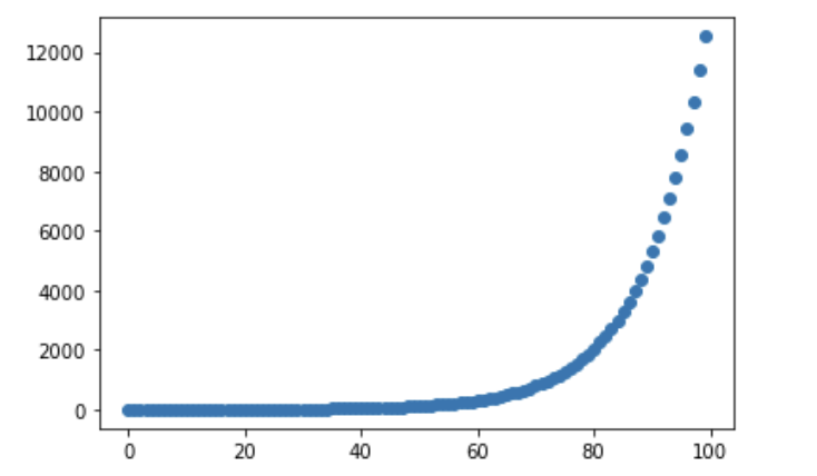
This formula highlights the exponential nature of compounded returns. Reminder: an exponential growth is when the time is the exponent $f: t \mapsto \lambda^t$.

When plotted for different timeframes, the exponential curve appears as showed below.

ret = .1
n = 100
f = lambda t:(1+ret)**t
plt.scatter(x=np.arange(n), y=[f(t) for t in range(n)])
plt.show()

Note: an interesting rule of thumb to find the moment when the wealth is doubled.

Annualization

Annualization refers to the computation of a 1-year return. Let $P_0$ be the initial price and $P_k$ the final price. $R_{annualized} = (\frac{P_k}{P_0})^{1/k}-1$ where $k$ is the number of years between $P_0$ and $P_k$. The formula can be deduced from the above compounding equation.

Portfolio returns

TWR

In the context of portfolio performance, the multiperiod return \(R_{t,k} = (R_{t}+1)*...*(R_{t-k+1}+1)-1\) is also called “time weighted return (TWR)”. A TWR is just about multiplying growth rate; it doesn’t consider cash flows. The naming “time weighted” means that equal weight is given to each sub-period’s return over time.

In case there are cash-flows, one way to compute the TWR is to remove them before computing the sub-period performance. E.g. every day, we substract the deposits and withdrawals from the portfolio valuation before computing the daily performance. We then do the cross product to have the final performance. That way, the cash flows don’t impact the performance. The below code illustrates the concept.

# daily valuations
data = {
        'dates':['2024-01-01','2024-01-02','2024-01-03','2024-01-04','2024-01-05'],
        'portfolio_value':[100,182,190,138,137],
        'deposits':[0,80,0,0,0],
        'withdrawals':[0,0,0,-50,-0]
        }
df = pd.DataFrame(data)
def TWR(df):
    df['daily_change'] = ((df['portfolio_value']-df['deposits']-df['withdrawals'])-df['portfolio_value'].shift())
    df['daily_change_pct'] = df['daily_change']/df['portfolio_value'].shift()
    portfolio_return = (1+df['daily_change_pct']).prod()-1
    return portfolio_return
print('{}%'.format(round(TWR(df)*100,2)))

The TWR is mostly used to compare fund performance. Hence, this return is widely used by fund managers.

MWR

When there are cash flows (i.e. inflows/outflows), it is common to use a “money weighted return (MWR)”. MWR adjusts the performance based on cash flows. See the Wealth Planning section for an example where the timing can impact the gains. The MWR is mostly used by individual investors.

2 common MWR are the internal rate of return and the modified Dietz method.

with:

• $A$ the starting amount of the portfolio.

• $PV$ is the present value of the portfolio.

import numpy_financial as npf
from pyxirr import xirr

# Relationship TWR / MWR
CF = [-100, 0, 0, 130]
twr = (130/100)**(1/3)-1
mwr = npf.irr(CF)
print(round(twr,2)==round(mwr,2)) # prints True

# XIRR when cash flows are non periodic (i.e. don't come regularly)
CF = [-100, -20, 130]
dates = ['2024-01-01','2024-02-01','2025-05-31']
mwr2 = xirr(dates, CF)
print(mwr2) # close to 5 percent (we invested 120 and got 130 after 2 years)

The IRR considers cash flows because the performance would change if we change the date of the cash flows (ceteris paribus).

Note: IRR is also equivalent to the YTM for bonds.

The difference between TWR and MWR (IRR) is well explained here.

The modified Dietz method is computed as such:

where

• $IV$ is the initial value of the portfolio

• $FV$ is the final value of the portfolio

• $F$ is the sum of all cash flows during the computation period

• $W_i$ is the weight of cash flow $i$ i.e. the time remaining before the end of the computation period

Note: the MDM needs to be annualized after computation.

The MDM has the advantage of being easy to compute i.e. without any optimisation algorithm (unlike the IRR). It is a good balance between accuracy and simplicity.