One simple approach to portfolio optimization is to not use any correlation matrix and rather focus on optimizing the investment ratio.
\[\max_{\omega_1, \omega_2} \quad \omega_1 + \omega_2\]With this problem, we want to make sure the maximum of our money is invested in financial products.
Matrix formulation
The package scipy.optimize.linprog allows to solve problems of the following form:
\[\begin{aligned} \min_x \quad c^Tx \\ \text{s.t.} \quad A_{ub} x \preccurlyeq b_{ub} \end{aligned}\]The curly symbol means that inequalities are componentwise. In other words, the inequalities hold for every component in the vectors.
In the context of portfolio optimization, $x$ are the weights that we allocate to each financial instrument:
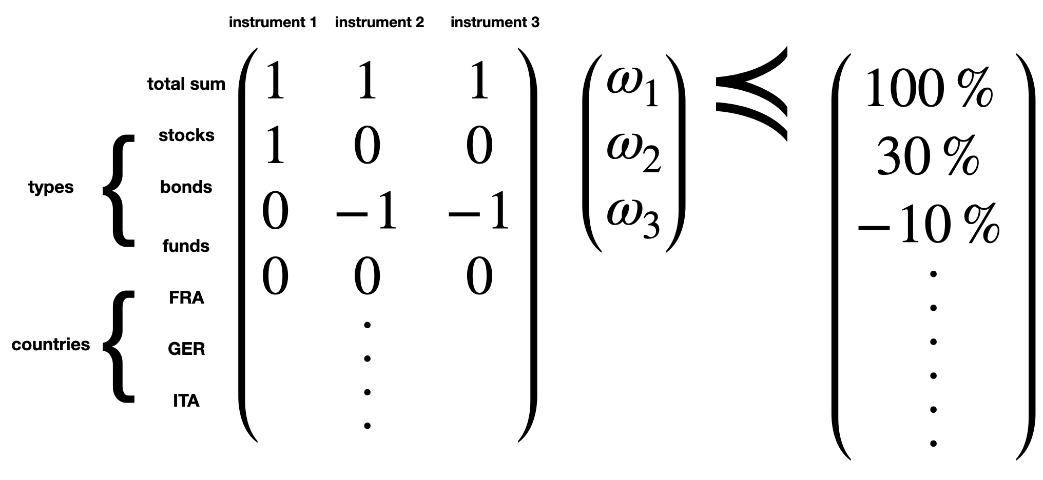
Note: we use negative numbers in the third line so that we have a lower bound. The third line is equivalent to $\omega_2 + \omega_3 \geq 10\%$.
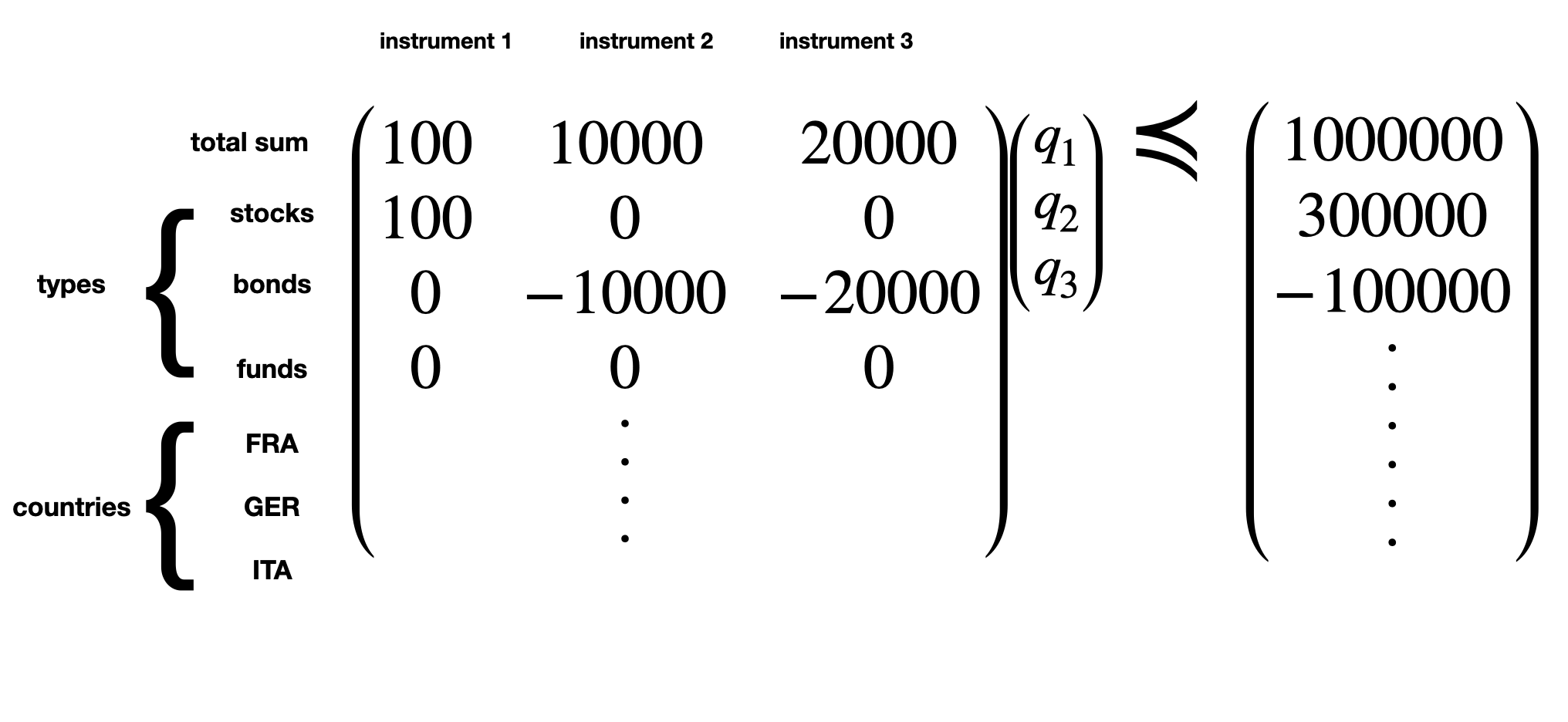
In order to take denomination into account, one can:
-
multiply $A_{ub}$ column-wise by the denomination (e.g. nominal if bond)
-
multiply $b_{ub}$ by the total amount to be invested
Below an example with $1,000,000$ as AUM:
Note: when using quantities, it’s important to weight by the denomination. The below example helps to understand the rationale.
$\max_{q_1, q_2} \quad q_1 + q_2$
$s.t. \quad 1 q_1 + 2 q_2 \leq 5$
In this first example, asset 1 will be inevitably preferred because $q_2$ is more weighted so gets bounded quicker. We can cancel this effect using the denomination also in the objective function:
$\max_{q_1, q_2} \quad q_1 + 2q_2$
$s.t \quad 1 q_1 + 2 q_2 \leq 5$
Asset class
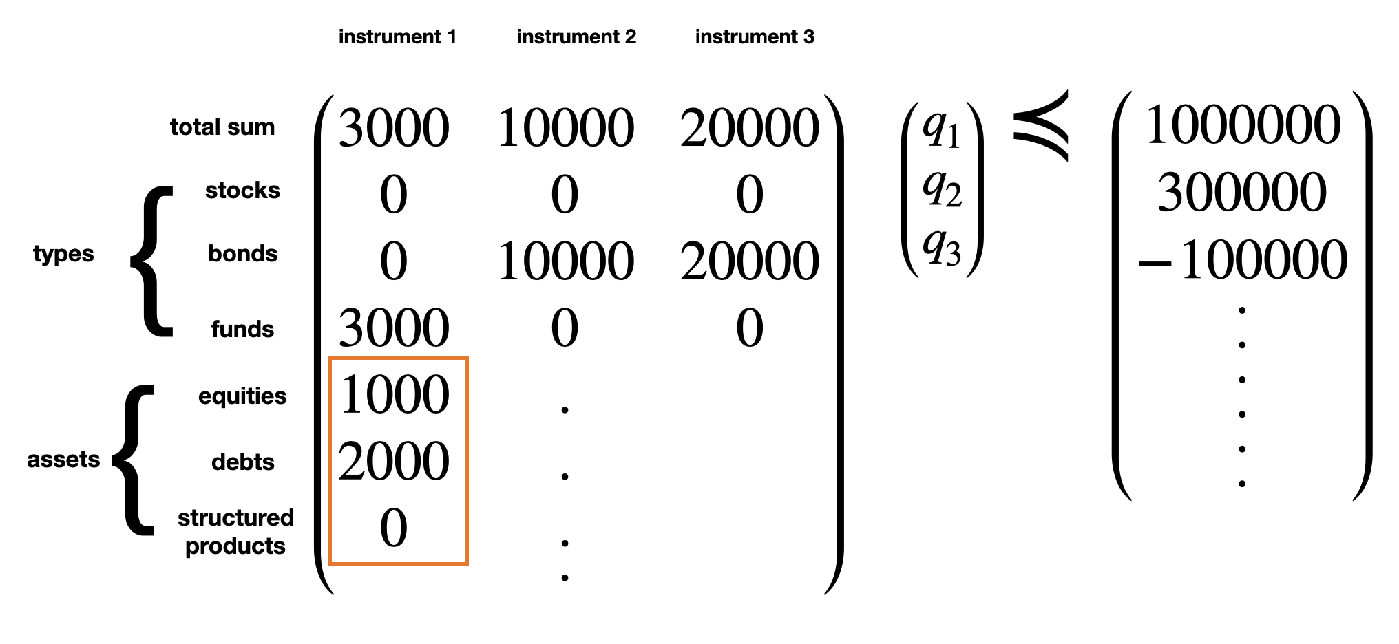
Funds have multiple asset class exposures. This can be easily handled using the right coefficient for the relevant dimension.
In the below example, instrument 1 is a fund with 1/3 of equities and 2/3 of debt (bonds).
Friction case
Transaction costs can be taken into account modifying the objective function. In the next example, we assume asset 1 has a denomination of 100 while asset 2 has a denomination of 10000.
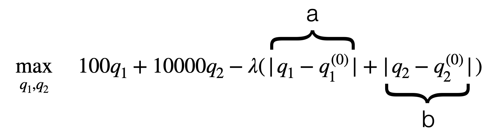
a) Approach 1: penalize quantities
\[\max_{q_1, q_2} \quad 100q_1 + 10000q_2 - \lambda(|q_1 - q_1^{(t-1)}| + |q_2 - q_2^{(t-1)}|)\]This approach penalizes every transaction the same. It may not be realistic since buying one stock at \$10 and buying one bond at $100,000 would likely not have the same absolute cost. Furthermore, since the objective is now to maximize the investment ratio AND to minimize the transaction costs, the model will favour instruments with higher denomination. E.g. bonds typically have a high denomination, hence would allow to quickly increase the investment ratio with a minimum transactions.
While the above is an important behaviour to keep in mind, considering that a solution would satisfy all constraints, one can say that we don’t really care whether instruments with high denomination are selected, as long as the constraints are satisfied.
Because the absolute function is not linear, one needs to rework the problem.
We can write the absolute function with a max:
\[a = |q_1 - q_1^{(0)}|\]$a = \max\{q_1 - q_1^{(0)}, q_1^{(0)} - q_1\}$
This implies:
$a \geq q_1 - q_1^{(0)}$
$a \geq q_1^{(0)} - q_1$
The constraints are written with the unknown variables at the LHS:
$q_1 - a \leq q_1^{(0)}$
$a + q_1 \geq q_1^{(0)}$
The similar can be done for b.
With $A$ and $b$ the matrices as defined above, the matrix formulation is:
\[\begin{pmatrix} A & 0 \\ -I_n & -I_n \\ I_n & -I_n \end{pmatrix} \preccurlyeq \begin{pmatrix} b \\ -q_n \\ q_n \end{pmatrix}\]b) Approach 2: penalize volume change
\[\max_{q_1, q_2} \quad 100q_1 + 10000q_2 - \lambda(100|q_1 - q_1^{(0)}| + 1000|q_2 - q_2^{(0)}|)\]The volume change can also be referred to “turnover”: it’s the total AUM that we buy/sell to end up with the new portfolio.
c) Approach 3: penalize any touch
\[\begin{aligned} \max_{q_1, q_2} \quad 100q_1 + 10000q_2 \\ \text{s.t.} \quad \unicode{x1D7D9}_{\{|q_1-q_1^{(0)}|>0\}}+\unicode{x1D7D9}_{\{|q_2-q_2^{(0)}|>0\}} \leq n_{hits} \\ \quad ... \end{aligned}\]In this last approach, we penalize any touch on a product. Intuitively, it is indeed reasonable to assume most of the fees come from the very first purchased unit. E.g. buying one stock of Bank of America costs USD 19 for the first stock, then 0.04 per additional stock.
We also cap the number of positions that are changed by $n_{hits}$. This allows to make sure the solution is reasonable and does not involve too many trades. One could iterate on this variable and stop when the problem becomes feasible; this would ensure to have a solution with a minimum number of changes.
One way to linearize the objective function is:
\[\begin{aligned} \max_{q_1, q_2, a, b} \quad 100q_1 + 10000q_2 +\lambda (a+b) \\ \text{s.t.} \quad \lambda = 0 \\ \quad a \in \{0,1\} \\ \quad b \in \{0,1\} \\ \quad a \geq \epsilon(q_1-q_1^{(0)}) \\ \quad a \geq \epsilon(q_1^{(0)}-q_1) \\ \quad b \geq \epsilon(q_2-q_2^{(0)}) \\ \quad b \geq \epsilon(q_2^{(0)}-q_2) \end{aligned}\]With $\epsilon$ a very small number.
The constraint $\lambda = 0$ is here so that the binary variables $a,b$ don’t play any role in the objective function and should be deduced w.r.t. the constraints (they need to be satisfied). We still mention them in the objective function as it’s required by the optimization package (scipy).
Case 1: we touch instrument 1 i.e. $|q_1-q_1^{(0)}|>0$
\[\begin{aligned} a \in \{0,1\} \\ a \geq \epsilon' \end{aligned}\]With $\epsilon’$ a very small but strictly positive number. This will have the effect of “activating” the binary constraint. In that case, the only possible value of $a$ is $1$. Thus, $a=1$.
Case 2: we don’t touch instrument 1 i.e. $|q_1-q_1^{(0)}|=0$
\[\begin{aligned} a \in \{0,1\} \\ a \geq 0 \end{aligned}\]Here, $a$ can be $0$ or $1$. We could encourage $a$ to be $0$ in making sure that we use a minimum number of transactions. Indeed, when $a=1$ it would count as a transaction so if there is actually no trade, it prevents the function to increase even more.
Let $h = \frac{1}{\epsilon}$ be a very large number. The matrix formulation is:
\[\begin{pmatrix} A & 0 \\ -I_n & -I_n*h \\ I_n & -I_n*h \end{pmatrix} \preccurlyeq \begin{pmatrix} b \\ -q_n \\ q_n \end{pmatrix}\]Note: this will have the effect to cap the quantity variations to $h$. Indeed, if $|q_1-q_1^{(0)}| > h$, the problem is infeasible. However, if $h$ is large enough, it is reasonable to say that this “cap effect” is not really a problem because buying/selling a very large number of units can be considered as an unusual move.
It is also possible to ensure a minimum conditional investment. This would allow to avoid having too small positions.
\[q \frac{p}{AUM} > M \unicode{x1D7D9}_{\{q \neq 0\}}\]Let’s now linearize the above inequality. We create a binary variable \(z = \unicode{x1D7D9}_{\{q \neq 0\}}\). Moving all unknown variables to the same side, the above translates to:
\[\begin{aligned} q \frac{p}{AUM} - M z \geq 0 \\ z \geq \epsilon q \\ z \in \{0,1\} \end{aligned}\]Similar to the above, $\epsilon$ is a very small but strictly positive number.
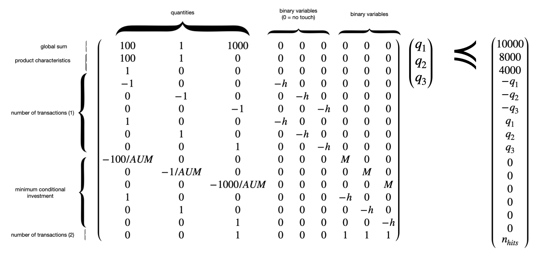
An example with 3 products, minimum number of trades and minimum conditional investment is showed below:
Weights for selection
To encourage the selection of certain products, one can use weights:
\[\max_{q_1, q_2} \quad \omega_1 100q_1 + \omega_2 10000q_2\]This would have the effect to push the gradient toward the variable with the highest weight as described in the theoretical part.
Note: it’s important to understand that using weights does not necessarily lead to less solutions. Indeed, we can find example where using weights actually increases the number of solutions.
Matrix simplification
When there are many constraints (rows) and instruments (columns), the optimization can take a long time. If the first constraint is: $p_1q_1 + p_2q_2 + … \leq AUM$, one can remove all redundant constraints $i$ (rows):
- constraints with maximal upper bound i.e. \(\{i, b_{ub}[i] = AUM, i \neq 0\}\)
E.g. in the below example, the constraint at index 1 is redundant (because of constraint at index 0) and can thus be removed:
\[\begin{pmatrix} 100 & 1000 & 200 \\ 100 & 1000 & 0 \\ 0 & 0 & 200 \\ \end{pmatrix} \preccurlyeq \begin{pmatrix} 10000 \\ 10000 \\ 3000 \end{pmatrix}\]- constraints with minimal lower bound i.e. \(\{ i, A_{ub}[i,j] \leq 0, \forall j\} \cup \{b_{ub}[i]=0 \}\)
E.g. in the below example, if we consider that all variables should be greater than $0$, the constraint at index 2 is redundant. Indeed, this constraint is equivalent to: $q_1 + q_2 \geq 0$, which is always true when $q_i \geq 0$.
\[\begin{pmatrix} 100 & 1000 & 200 \\ 100 & 1000 & 0 \\ -100 & 0 & -200 \\ \end{pmatrix} \preccurlyeq \begin{pmatrix} 10000 \\ 10000 \\ 0 \end{pmatrix}\]