Geometric representation

To better understand an optimization problem, it can be useful to see it geometrically.

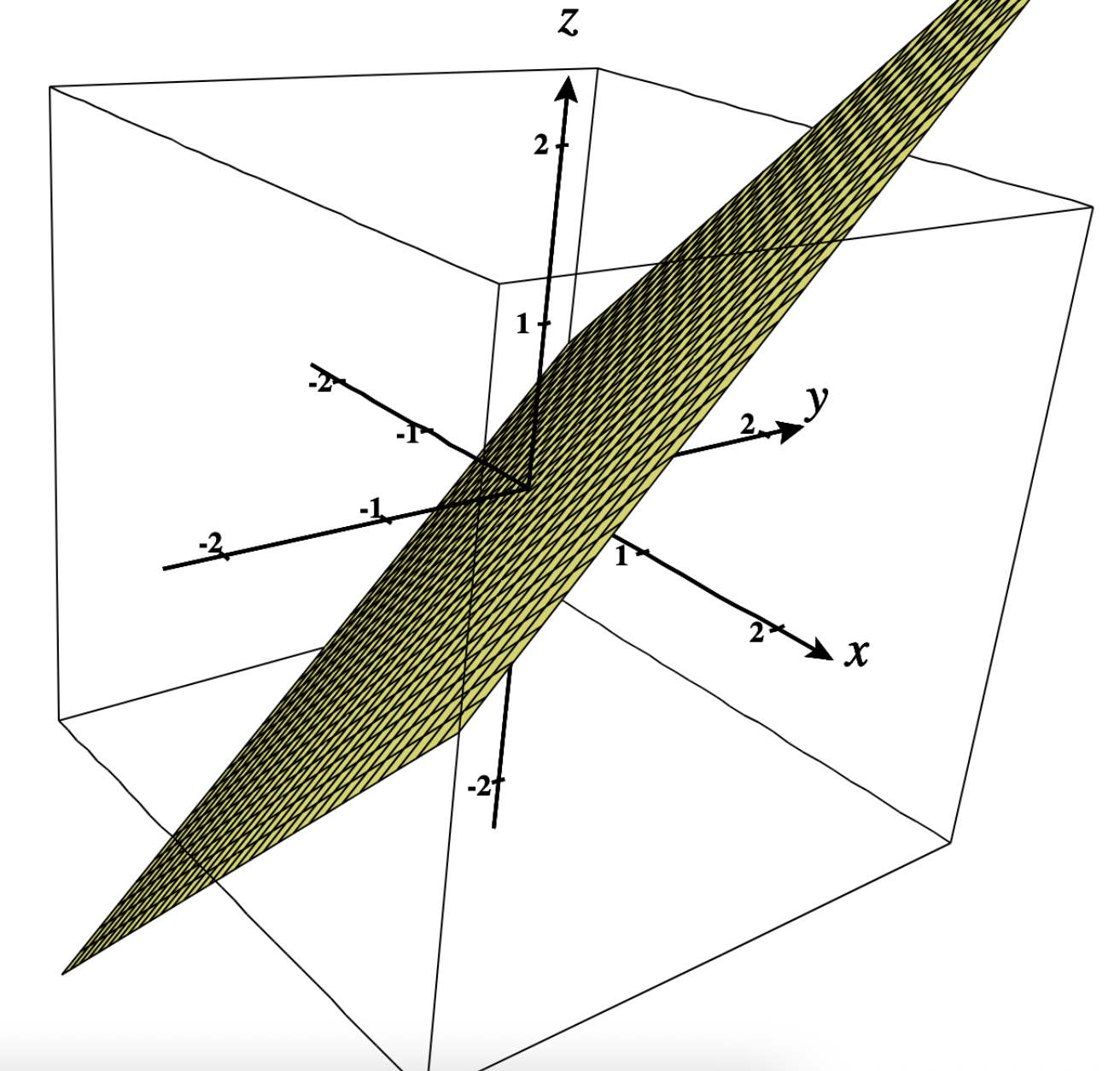
Example: objective function $f(x,y) = x+y$.

This problem is linear, since it’s the equation of a hyperplane $z = x+y => z-x-y =0$.

Reminder: a hyperplane has a linear equation: $a_1x_1 + … + a_nx_n = b$. Visually, a plane is a subspace whose dimension (actually, degrees of freedom) is one less than that of its ambient space. To draw the plane $z-x-y =0$, one can choose a variable that would be the dependent variable in order to have only 2 degrees of freedom. Here, it makes sense to choose $z$ as dependent variable since $x$ and $y$ are clearly the independent variables in the above problem (note: independent variables are the answer to the question: “what variables move first?”). The hyperplane can thus be represented in finding $z$ for various values of $x$ and $y$. We can thus represent this hyperplane in 3D (plot from c3d):

Now to understand the behaviour of $f$ when it is maximized, one can test increasing values of $z$. For each value of $z$, the resulting equation has only 1 degree of freedom and can thus be drawn in 2D. In the below picture, we plot the function for $z=1, 2, 3$ (plot from desmos) with the gradient represented by arrows (see details on gradient in the next section):

Let’s now consider $z = x + 2y$. Plotting $z=1,2,3$ gives:

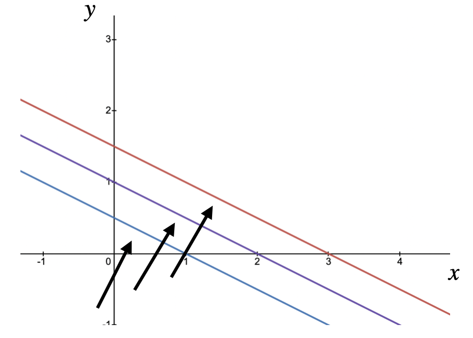
We can thus deduce that the gradient moves toward $y$ when weighting more $y$.

In other words, an optimization problem of the form $f(x,y) = x+2y$ would put a larger value on $y$ than on $x$ (ignoring constraints).

Reminders on gradient

The gradient of a function is a vector with all the function’s partial first derivatives as components.

\[\begin{align*} \nabla f = \begin{bmatrix} \frac{\partial f}{\partial x_1} \\ ~ \\ \frac{\partial f}{\partial x_2} \\ ~ \\ \frac{\partial f}{\partial \lambda} \end{bmatrix} \end{align*}\]

It is also the “direction and rate of fastest increase”. Let’s consider a hill as shown below. At any point, the gradient is always the vector pointing to the top (image from here):

As mentioned above, the gradient can be deduced in increasing the value of $f(x,y)$. Below is an example with $f(x,y) = xy$ where we plot $xy=1$, $xy=2$, $xy=3$ (plot from desmos):

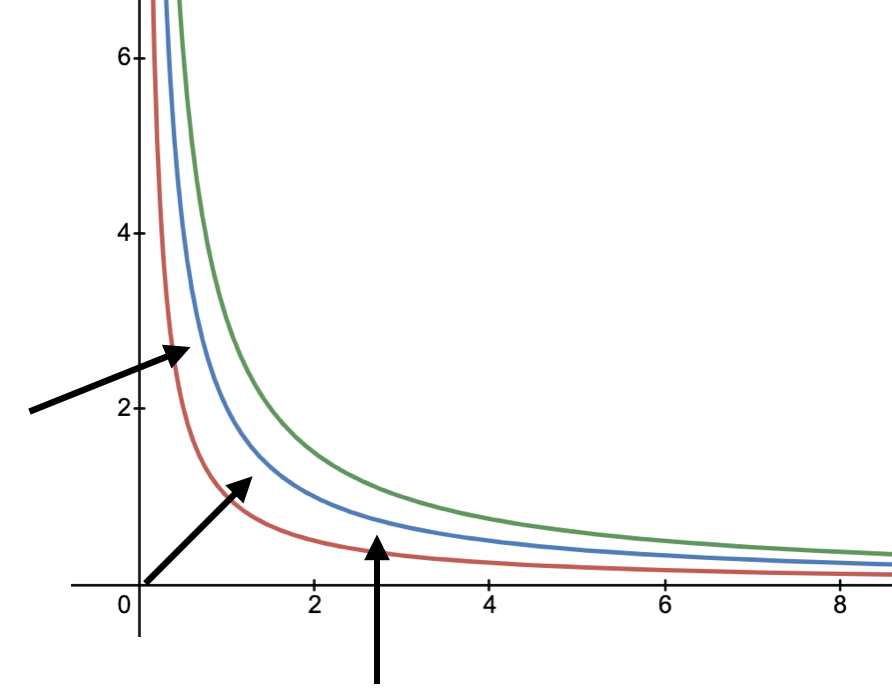
One can confirm the gradient on elsenaju:

Case without constraint: FOC and SOC

First order condition (FOC): $x^*$ local optimum => \(\nabla f(x^*) = 0\)

Note: when \(\nabla f(x^*) = 0, x^* \text{ is called critical or stationary point}\).

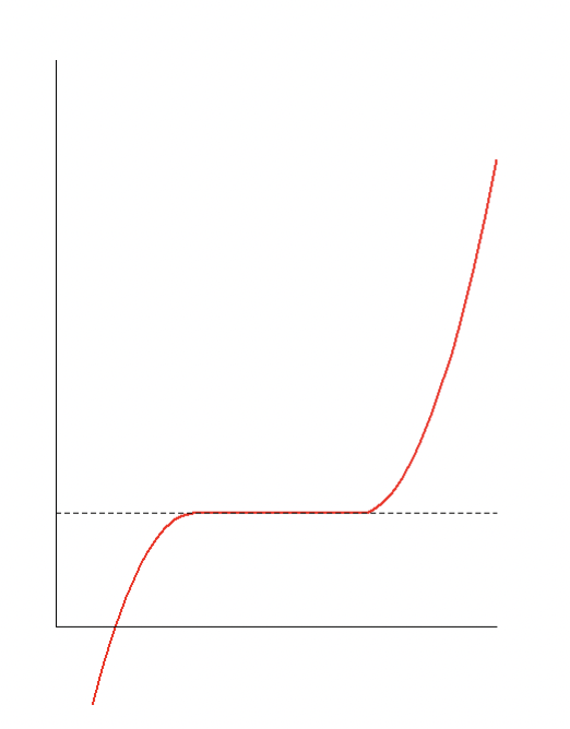
Warning: FOC are necessary conditions but not sufficient. In the below figure \(\nabla f(x^*) = 0\) but $x^*$ is not a optima:

Second order conditions (SOC): $f^{2}(x^*) \geq 0$

If \(x^{*}\) satisfies both FOC and SOC (strictly i.e. \(f^{2}(x^{*}) > 0\)) then \(x^{*}\) is an optimum.

Case with equality constraints: Lagrange method

\[\text{optimise } f(x)\] \[\text{s.t. }h_j(x) = 0\]

At any local maxima (minima) of the function evaluated under equality contraints, then the gradient of the function (at that point) can be expressed as a linear combination of the gradients of the constraints, with the Lagrange multipliers acting as coefficients.

\[\nabla f(x^*) =\lambda^T \nabla g(x^*)\]

Gradient of the function = linear combination of gradients of the constraints (coefficients = Lagrange multipliers).

We can illustrate this definition using again the analogy with the hill as above. The constraint is defined as the squared area cutting the hill. We can see that the optimum point is found where \(\nabla f(x^*)=\lambda^T \nabla g(x^*)\) (thick arrow):

\(\nabla f(x^*)=\lambda^T \nabla g(x^*)\) => \(\nabla f(x^*) - \lambda^T \nabla g(x^*) = 0~~~(E)\)

In practice, to solve the above problem, the Lagrange method consists in forming the Lagrangian function $\mathcal{L}(x, \lambda) = f(x)-\lambda g(x)$. Then, at each local maximum (minimum), based on $(E)$, all partial derivatives should be zero.

Example:

\[\text{optimise }y+x^2\] \[\text{s.t. } x+y=1\]

$\mathcal{L}(x, y, \lambda) = y+x^2+\lambda_1(x+y-1)$

At optimum:

$\frac{\partial\mathcal{L}}{\partial x}=0~~~~~$ (1)

$\frac{\partial\mathcal{L}}{\partial y}=0~~~~~$ (2)

$\frac{\partial\mathcal{L}}{\partial\lambda_1}=0~~~~$ (3)

(2) => $\lambda_1 = -1$ (1) => $x = \frac{1}{2}$ (3) => $y = \frac{1}{2}$ \

The solution is $x^* = \frac{1}{2}$, $y^* = \frac{1}{2}$.

Problem with equality and inequality constraints: KKT conditions

The KKT conditions generalize the Lagrange method with inequality constraints.

\[\text{optimise } f(x)\] \[\text{s.t. } g_i(x) \leq 0\] \[~~~~~~h_j(x) = 0\]

$\mathcal{L}(x, \mu, \lambda) = f(x) + \mu^T g(x) + \lambda^T h(x)$

$g$ are the inequality constraints.

$h$ are the equality constraints.

If $x^*$ is a local optimum, then the following conditions hold:

(1) Primal feasability

$h_j(x^*) = 0~~\forall j$

$g_i(x^*) \leq 0~~\forall i$

Intuitively, the feasible solutions are candidates that satisfy all constraints. If there exists a feasible set, it means there is (at least) one solution to the problem.

(2) Dual feasability

$\lambda_i \geq 0~~\forall i$

From wikipedia: “duality is the principle that optimization problems may be viewed form either of two angles: the primal problem or the dual problem. If the primal is a minimization problem then the dual is a maximization problem. In general, the optimal values of the primal and dual problems need not to be equal.”

(3) Complementary slackness

$\mu_i g_i(x^*) = 0~~\forall i$

(4) Stationarity

\[\nabla f(x^*) + \sum_j \mu_j \nabla g_j(x^*) + \sum_i \lambda_i \nabla h_i(x^*) = 0\]

Warning: KKT conditions are necessary but not sufficient! Example here (page 21).

Global or local

To find out whether a solution is global, one can look at the following aspects:

• convexity: $f$ convex => a local optimum is also global

• coercivity

This document summarizes well all different cases as well as the necessary/sufficient conditions.