A quadratic function is a polynomial of degree two in one or more variables (source wikipedia).
In one dimension:
\[f(x) = ax^2 + bx + c \quad a \neq 0\]Warning: a quadratic function is not necessarily convex!
Portfolio optimization
Generic formulation
In the context of portfolio optimization under the mean-variance theory, we want to minimize the portfolio variance and maximize its return.
Constraints are set in a way that we prevent shortselling and that all individual investments are below a threshold (to avoid bulk risk - also called concentration risk).
\[\begin{aligned} \min_\omega \quad \omega^T\Sigma \omega -\omega^T \mu \\ \text{s.t.} \quad \sum_i x_i = 1 \\ \quad x_i \geq 0 \\ \quad x_i \leq m \\ \end{aligned}\]Efficient frontier
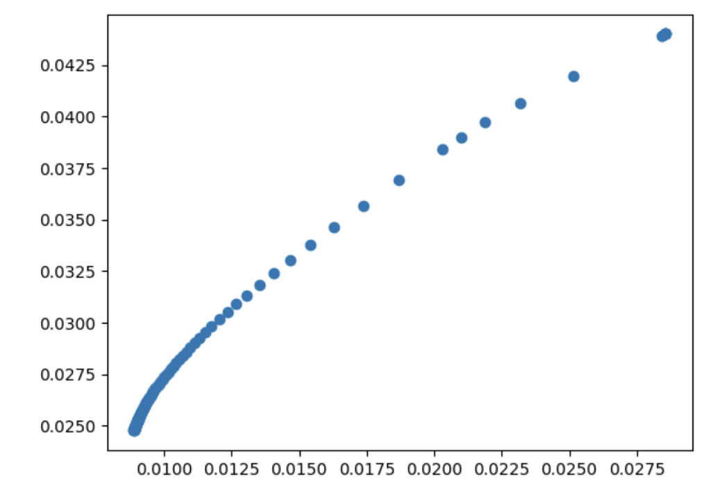
To find out all optimal portfolios, we introduce a risk aversion coefficient $\lambda$.
\[\begin{aligned} \min_\omega \quad \frac{\lambda}{2}\omega^T\Sigma \omega -\omega^T \mu \\ \text{s.t.} \quad \sum_i x_i = 1 \\ \quad x_i \geq 0 \\ \quad x_i \leq m \\ \end{aligned}\]In order to find the frontier, we optimize portfolios for several aversion coefficients. The higher the aversion coefficient, the lower would be the return and the volatility of the portfolio.
Implementation
CVXOPT is a great package with a specific module for quadatric programming. Here a detailed example using the package.
Constraints are defined as such:
\[Ax = b\] \[Gx \preccurlyeq h\]The curly symbol means that inequalities are componentwise. In other words, the inequalities hold for every component in the vectors.
Example: let’s consider a portfolio with 3 assets. The constraints $\omega_1 \leq 40\%, ~~ \omega_2 \geq 20\%$ would required to use the following matrices:
\[G = \begin{pmatrix} 1 \\ -1 \\ 0 \end{pmatrix}, \quad h = \begin{pmatrix} 0.4 \\ -0.2 \\ 0 \end{pmatrix}\]
# Computing the efficient frontier

# ******** Creating synthetic data for illustration *******

# Bond IG
mu_1 = 0.02
sigma_1 = 0.01
# Note: those figures generally come from
# an external model (e.g. risk factor model)

# Equities
mu_2 = 0.05
sigma_2 = 0.04

# Hedge funds
mu_3 = 0.03
sigma_3 = 0.02

# monthly returns
returns_1 = np.random.normal(mu_1/12, sigma_1/np.sqrt(12), size=10000)
returns_2 = np.random.normal(mu_2/12, sigma_2/np.sqrt(12), size=10000)
returns_3 = np.random.normal(mu_3/12, sigma_3/np.sqrt(12), size=10000)

corr = np.corrcoef([returns_1, returns_2, returns_3])
var = np.diag([sigma_1, sigma_2, sigma_3])
# Note: the variance needs to be the right unit / doesn't mind for the correlation
cov = np.dot(np.dot(corr, var), var)

# ******** Optimization *******

n = 3 # in this example we use 3 assets only
max_weight = 0.7

r = matrix(np.array([mu_1, mu_2, mu_3]))
Q = matrix(cov)

# Equality constraints
A = matrix(np.ones(n)).T
b = matrix(1.0)

# Inequality constraints
G = matrix(np.concatenate([-np.eye(n), np.eye(n)]))
h = matrix(np.concatenate([np.zeros(n), np.ones(n)*max_weight]))

# ******** Aversion coefficient *******

N = 100
lambdas = [t*10 for t in range(N)]

# ******** Optimization *******

# For each aversion coefficient, we find optimal weights

options['show_progress'] = False
sol = [np.array(qp(lmbda / 2 * Q, -r, G, h, A, b)['x']).flatten() for lmbda in lambdas]
options['show_progress'] = True

# we compute the expected return/volatility for each portfolio
exp_ret_list = [np.dot(w_iter.T, r)[0] for w_iter in sol]
exp_vol_list = [np.sqrt(np.dot(np.dot(w_iter.T, cov), w_iter)) for w_iter in sol]

plt.figure()
plt.scatter(exp_vol_list, exp_ret_list)
plt.show()
Transaction costs
Transaction costs can be taken into account as such:
\[\min_\omega \quad \frac{\lambda}{2}\omega^T\Sigma \omega -\omega^T \mu + z(\sum \Delta \omega_i^- + \sum \Delta \omega_i^+)\]Where $\Delta \omega_i^+$ (resp. $\Delta \omega_i^-$) is the increase (resp. decrease) in weight for instrument $i$. $z$ is the transaction penalty coefficient i.e. the fee percentage. E.g. 0.01 is 1% fees applied on the total transaction amount $(\sum \Delta \omega_i^- + \sum \Delta \omega_i^+$).
The problem can be rewritten:
\[\min_W \quad \frac{\lambda}{2}W^TC W -W^T q\]Where: \(W = \begin{pmatrix} \omega_1 \\ \omega_2 \\ \Delta \omega_1^- \\ \Delta \omega_2^- \\ \Delta \omega_1^+ \\ \Delta \omega_2^+ \\ \end{pmatrix}\)
$C$ and $q$ can be derived respectively from $\Sigma$ and $\mu$. Below is an illustration with 2 assets only.
\[C = \begin{pmatrix} \Sigma & & 0 & 0 & 0 & 0 \\ & & 0 & 0 & 0 & 0 \\ 0 & 0 & 0 & 0 & 0 & 0 \\ 0 & 0 & 0 & 0 & 0 & 0 \\ 0 & 0 & 0 & 0 & 0 & 0 \\ 0 & 0 & 0 & 0 & 0 & 0 \end{pmatrix}\] \[q = \begin{pmatrix} \mu \\ \\ -z \\ -z \\ -z \\ -z \end{pmatrix}\]We illustrate the changes with 2 variables only:
\[\min_\omega \quad \frac{\lambda}{2}W^T \begin{pmatrix} c_{11} & c_{12} & 0 & 0 & 0 & 0 \\ c_{21} & c_{22} & 0 & 0 & 0 & 0 \\ 0 & 0 & 0 & 0 & 0 & 0 \\ 0 & 0 & 0 & 0 & 0 & 0 \\ 0 & 0 & 0 & 0 & 0 & 0 \\ 0 & 0 & 0 & 0 & 0 & 0 \end{pmatrix} W - W^T \begin{pmatrix} \mu_1 \\ \mu_2 \\ -z \\ -z \\ -z \\ -z \end{pmatrix}\]Implementation
We assume only 2 assets.
When using CVXOPT, the constraints are expressed the same:
\[Gx \preccurlyeq h\]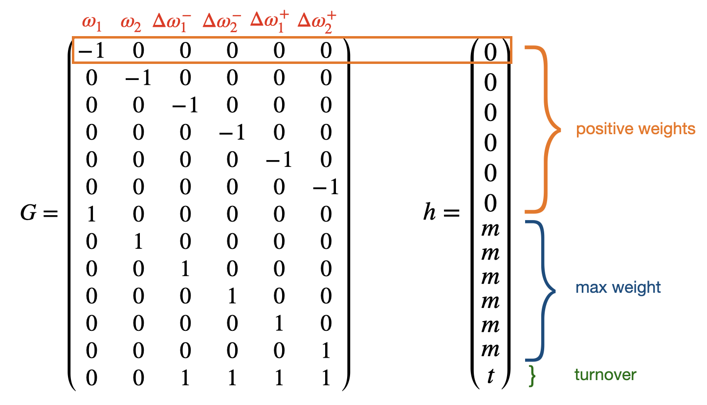
The last equation accounts for the maximum possible turnover i.e. if we sell everything and buy an entire new portfolio (200% change): $\Delta \omega_1^-+\Delta \omega_2^-+\Delta \omega_1^++\Delta \omega_2^+ = 2$
\[Ax = b\]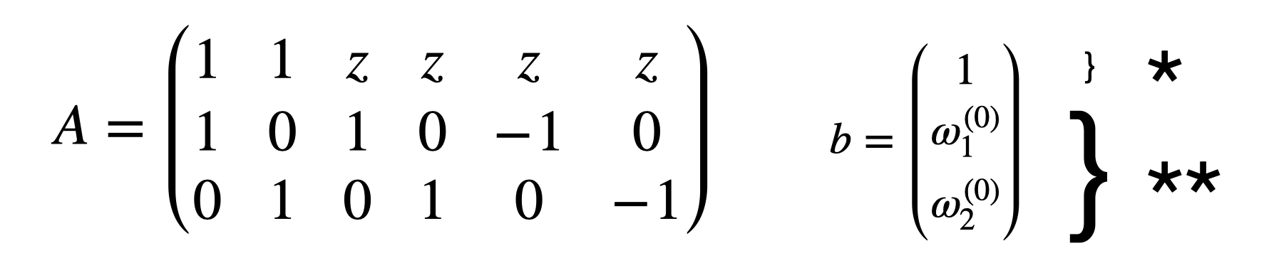
Equation $*$ accounts for the fact that the total wealth is used to invest in the instruments AND pay the fees associated with any change: $\omega_1+\omega_2+z(\Delta \omega_1^-+\Delta \omega_2^-+\Delta \omega_1^++\Delta \omega_2^+) = 1$. When $z \neq 0$, we have $\sum w_i < 1$, which may seem counterintuitive. However, it makes sense because the remaining wealth allows to pay the fees.
Equation $**$ accounts for the old weights. For the first row: $\omega_1+\Delta \omega_1^–\Delta \omega_1^+ = \omega_1^{(0)}$. The equation becomes clearer when expressed as such: $\omega_1 = \omega_1^{(0)}-\Delta \omega_1^-+\Delta \omega_1^+$.
From weights to quantities
In portfolio optimization, it’s common to work with weights rather than quantities. We define the following terminology:
-
Theoretical weights are weights given by a model e.g. Markowitz: $\omega_{theo} = \omega_{model}$.
-
Real weights are weights reflecting the proportions in which the model user is actually investing.
-
$AUM$ is the total portfolio amount.
In practice, it’s not possible to have the theoretical weights fully aligned with the real weights if the unit sizes are not taken into account in the modeling part.
Note: unit sizes can be computed differently depending on the product type:
-
Stock: unit size = current price
-
Bonds: unit size = current price (%) * nominal
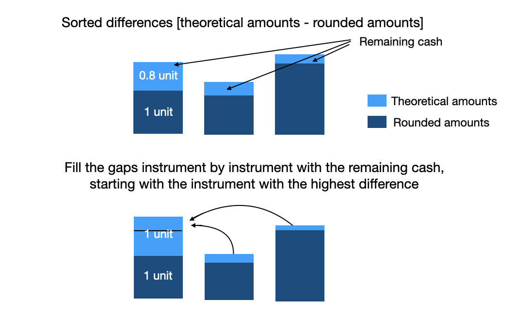
In order to have the minimum difference between the theoretical and real weights, one can think about the following logic:
- (1) Compute theoretical amounts
- (2) Compute theoretical quantities
- (3) Compute rounded quantities. We round to the lower integer since we want to make sure we can’t invest more than the AUM.
- (4) Compute rounded amounts
- (5) Compute the difference [theoretical amounts - rounded amounts] for each instrument. In doing so, we can identify what instruments have rounded amounts that are far from the theoretical amounts. We will then try to improve the situation starting with those instruments first.
-
(6) Rank instruments according to D in descending order
-
(7) Compute the remaining cash
- (8) For each instrument, we try to buy one more unit with the remaining cash, starting with the one with the highest difference D. At each step, the remaining cash is updated.
The below schema illustrate the logic :
def weights_to_quantities(aum, weights_theo_arr, nominals_arr, instrument_names):

    # (1) Compute theoretical amounts
    amounts_theo = weights_theo_arr*aum

    # (2) Compute theoretical quantities
    quantities_theo = amounts_theo/nominals_arr

    # (3) Compute rounded quantities
    quantities_round = np.floor(quantities_theo)

    # (4) Compute rounded amounts
    amounts_round = quantities_round*nominals_arr

    # (5) Compute the difference D=[amounts_theoretical-amounts_rounded]
    D = amounts_theo-amounts_round

    # (6) Rank instruments according to D in descending order
    diff_sorted_idx = (-D).argsort()

    # (7) Compute the remaining cash
    remaining_cash = aum-np.sum(amounts_round)
    print('Remaining cash after rounding: {}'.format(remaining_cash))

    # (8) For each instrument, try to buy one more unit with the remaining cash,
    # starting with the one with the highest difference D
    quantities_real = quantities_round.copy()
    for diff_idx in diff_sorted_idx:
        if remaining_cash>=nominals_arr[diff_idx]:
            print('-> We can buy one more unit of instrument {}'.format(diff_idx))
            quantities_real[diff_idx] = quantities_real[diff_idx]+1
            remaining_cash = aum-np.sum(quantities_real*nominals_arr)

    print('Amount of cash that can\'t be invested: {}'.format(remaining_cash))
    weights_real = quantities_real*nominals_arr/aum

    # Display
    plt.bar(instrument_names, weights_theo_arr, alpha=.5, label='theoretical weights')
    plt.bar(instrument_names, weights_real, alpha=.5, label='final weights')
    plt.legend()
    plt.xticks(rotation=45)
    plt.show()

    return quantities_real, weights_real