Variance

Variance theoretical formula: $\mathbb{V}[X] = \mathbb{E}[(X-\mathbb{E}[X])^2]$

Variance empirical formula: $var_n(x) = \frac{1}{n} \sum_{i=1}^n (x_i - \bar x)^2$

Variance (sample) empirical formula: $var_n(x) = \frac{1}{n-1} \sum_{i=1}^n (x_i - \bar x)^2$

The sample variance is larger than the population variance so that it takes into account of additional uncertainty .

Volatility

Volatility empirical formula: $\sigma = \sqrt{var_n(x)}$

The volatility is most often computed from the returns. Intuitively, it represents the “typical variation”.

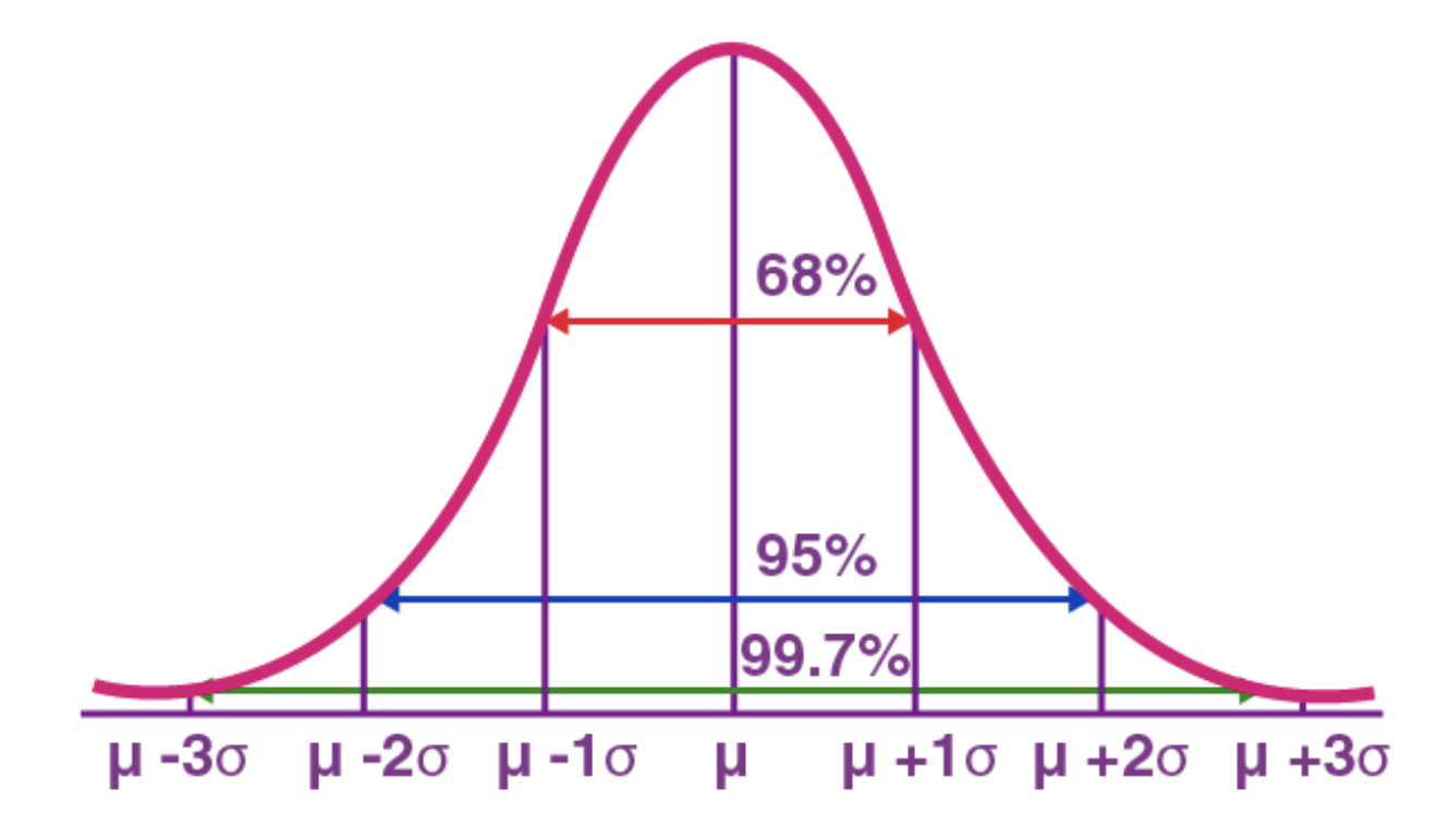
If the variable is normally distributed, the below figure is important to have an order of magnitude:

Volatility is important in algorithmic trading since a good trade should be profitable after fees deduction. Hence the asset move should be large enough to pay the fees.

Variance of a portfolio

Let’s find the formula starting with a small portfolio with number of assets = 2.

\[R_p = \omega_1 R_1 + \omega_2 R_2\] \[\begin{align*} \mathbb{V}[R_p] &= \mathbb{V}[\omega_1 R_1 + \omega_2 R_2] \\ &= \omega_1^2\mathbb{V}[R_1]+\omega_2^2\mathbb{V}[R_2]+2\omega_1\omega_2Cov(R_1,R_2) \quad \quad \quad (*)\\ &= (\omega_1~~\omega_2) \begin{pmatrix} \mathbb{V}[R_1] & Cov(R_1, R_2) \\ Cov(R_1, R_2) & \mathbb{V}[R_2] \end{pmatrix} \begin{pmatrix} \omega_1 \\ \omega_2 \end{pmatrix} \\ \end{align*}\]

We can thus generalize the formula:

\[\sigma_p^2= \omega^T \Sigma \omega\]

$(*)$ can also be written using the correlation coefficient $\rho$:

$\mathbb{V}[R_p] = \omega_1^2\mathbb{V}[ R_1]+\omega_2^2\mathbb{V}[R_2]+2\omega_1\omega_2 \sqrt{\mathbb{V}[ R_1]} \sqrt{\mathbb{V}[ R_2]} \rho_{1,2}$

From this equation, we can see that the portfolio variance is maximized when $\rho_{ij}=1$ (perfect correlation). It is minimal when $\rho_{ij}=-1$ i.e. when assets are perfectly negatively correlated. We notice than when $\rho_{ij}=1$, we have $\mathbb{V}[R_p] = (\omega_1\sigma_1 + \omega_2\sigma_2)^2$. This result shows that when assets are perfectly correlated, the volatility of a portfolio is the weighted average of the assets’ volatilities.

We could also compute the portfolio volatility using the correlation matrix. This is useful for better interpretation (it’s easier to double check a correlation matrix than a covariance matrix).

\[\sigma^2_p = \omega^T S C S \omega\]

where $C$ is the correlation matrix and $S$ the standard deviation (diagonal) matrix:

\[S = \begin{pmatrix} \sigma_1 & \\ & \ddots & \\ & & \sigma_n \end{pmatrix}\]

Warning: make sure the standard deviations and not the variances are used in $S$. It’s also important to make sure those standard deviations are of the right unit (e.g. annualized).

Annualization

Annualize refers to converting a short-term number, such as an investment return or interest rate, into an annual rate.

Note:

• annual volatility: computed on several years e.g. 2020, 2021, 2022.

• annualized volatility: computed on one year based on monthly or daily returns.

In practice, we use the annualized volatility because we don’t have the annual returns of a large sample of years.

Let us say we want to compute the annualized standard deviation based on the monthly returns. When returns are continuous:

\[\begin{align*} var(r_{2020}) &= var(r_{jan, 2020}+...+r_{dec, 2020}) \quad \text{Reminder: when returns are continuous: } r_{0,2} = r_{0,1}+r_{1,2}\\ &= var(\sum_{i=1}^{12}r_{i, 2020}) \\ &= \sum_{i=1}^{12}var(r_{i, 2020}) \quad \text{assuming independent returns}\\ &= 12var(r_{monthly}) \\ \end{align*}\]

Thus, we have:

\[\sigma_{annualized} = \sqrt{12}\sigma_{monthly}\]

Similarly, assuming trading happens all day long:

\[\sigma_{annualized} = \sqrt{365 * var_{daily}(x)} = \sqrt{365} \sigma_{daily}\]

Examples

• VIX: 15-20% (typical level in normal market environment).

Note: the VIX is a measure of the expected equity volatility.

• BTCUSD: 20% monthly (2019).

• BTCUSD: 84% annualized daily (2021).

• BTCUSD: 0.53% hourly (October 2022).

• XRPUSD: 1.17% hourly (October 2022).