European call
\[\text{payoff} = (S_T-K)^+\]import numpy as np
S0 = 100
r = .05
sigma = .2
T = 1/2
n_steps = 100
dt = T/n_steps
n_paths = 100000
St = np.zeros((n_paths, n_steps))
St[:,0] = S0
K = 110
for t in range(n_steps-1):
eps = np.random.normal(0,1,n_paths)
St[:,t+1] = St[:,t]*np.exp((r-sigma**2/2)*dt+sigma*eps*np.sqrt(dt))
path_no_exercise_idx = np.where(St[:,-1]<K)[0]
payoffs = St[:,-1]-K
payoffs[path_no_exercise_idx] = 0
price = np.mean(payoffs)*np.exp(-r*T)
print(price)
The above prints ~$2.88$. When n_steps tends to infinity, the price should tend to the theoretical value that is given by the Black-Scholes formula.
Barrier: up and out
\[\text{payoff} = \unicode{x1D7D9}_{\{ \tau(b) > T \}} (S_T-K)^+\]Where \(\tau(b) = \inf \{t_i : S_{t_i} > b \}\)
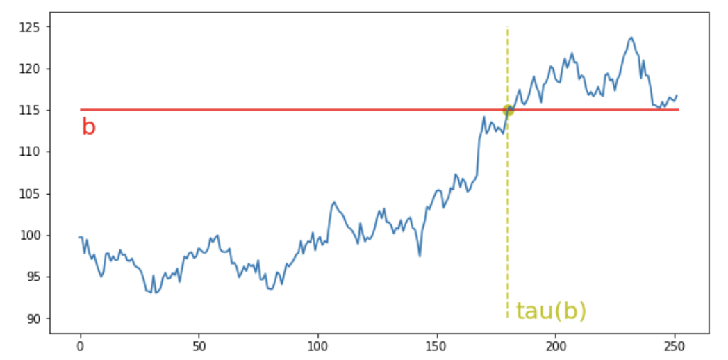
$\tau(b)$ is the first time the asset increases higher than the barrier level $b$. The indicator function in the payoff shows that the option can be exercised if this time happens after expiration.
import numpy as np
S0 = 100
r = .05
sigma = .2
T = 1/2
n_steps = 100
dt = T/n_steps
n_paths = 10000
St = np.zeros((n_paths, n_steps))
St[:,0] = S0
barrier = 130
K = 110
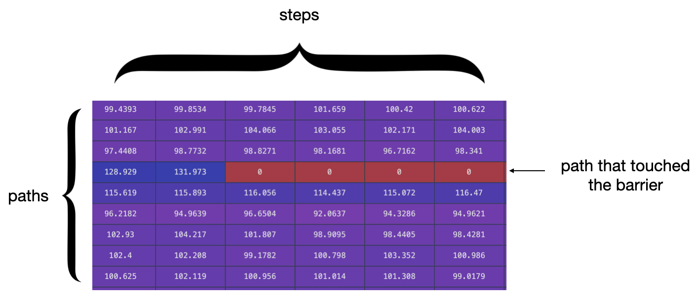
for t in range(n_steps-1):
# we identify the paths where the barrier is touched
# if the barrier is touched, the payoff will be zero
idx_barrier_knocked = np.where(St[:,t]>barrier)[0]
St[idx_barrier_knocked,t+1] = 0
# if the barrier is not touched, we simulate the next
# step
idx_barrier_not_knocked = np.array([i for i in range(n_paths) if i not in idx_barrier_knocked])
eps = np.random.normal(0,1,len(idx_barrier_not_knocked))
St[idx_barrier_not_knocked,t+1] = St[idx_barrier_not_knocked,t]*np.exp((r-sigma**2/2)*dt+sigma*eps*np.sqrt(dt))
# for path_idx in range(n_paths):
# plt.plot(np.arange(n_steps), St[path_idx])
# plt.hlines(y=barrier, xmin=0, xmax=n_steps)
path_no_exercise_idx = np.where(St[:,-1]<K)[0]
payoffs = St[:,-1]-K
payoffs[path_no_exercise_idx] = 0
price = np.mean(payoffs)*np.exp(-r*T)
print(price)
This prints ~$1.4$. Explanations: when a barrier is touched, the payoff is zero. Thus, compared to a vanilla call, the final list of values that we average contain more zeros. Those zeros tend the average toward zeros, hence reducing the final price.
Digital option
\[\text{payoff} = \unicode{x1D7D9}_{\{S_T > K\}}\] \[price = \frac{1}{100} \mathcal{N}(d_2)\]$\mathcal{N}(d_2)$ is the probability for $S_T$ to end above $K$.