A geometric Brownian motion is a special case of SDE. The following equation is the informal equation of the geometric Brownian motion:
\[dS_t = \mu S_t dt + \sigma S_t dB_t\]Note: “geometric” because increments $S_t$ are multiplied by another variable $dB_t$.
Returns
Thanks to Itô’s lemma we can solve the SDE. The following equation is the informal solution to the GBM’s equation:
\[d \ln S_t = (\mu - \frac{\sigma^2}{2}) dt + \sigma dW_t\]This equation is still in the informal form. To implement such process we need to find the formal form. This can be done by integrating over a specific interval w.r.t. the variable we want to remove ($t$ here).
When integrating over $[0,t]$:
LHS: $\int_0^t d \ln S_t = [x]_{\ln S_0}^{\ln S_t} = \ln S_t - \ln S_0 = \ln \frac{S_t}{S_0}$
RHS: $\int_0^t \Big( (\mu - \frac{\sigma^2}{2}) dt + \sigma dW_t \Big) = \int_0^t (\mu - \frac{\sigma^2}{2}) dt + \int_0^t \sigma dW_t = (\mu - \frac{\sigma^2}{2}) [x]_0^t + \sigma [x]_{W_0}^{W_t} = (\mu - \frac{\sigma^2}{2}) t + \sigma W_t$
Since $W_t \sim \mathcal{N}(0,\sqrt t^2), W_{t+\Delta t}-W_t \sim \mathcal{N}(0,\sqrt t^2+ \sqrt{\Delta t}^2 - \sqrt{t}^2)$ i.e. $W_{t+\Delta t}-W_t \sim \mathcal{N}(0,\sqrt{\Delta t}^2)$
=> $W_{t+\Delta t}-W_t = \epsilon \sqrt{\Delta t} \quad$ where $\epsilon \sim \mathcal{N}(0,1)$
We finally obtain the formal solution to the GBM’s equation (recursive version):
\[\ln \frac{S_{t+\Delta t}}{S_t} = (\mu - \frac{\sigma^2}{2}) \Delta t + \sigma \epsilon \sqrt{\Delta t} \quad (*)\]We can see that GBM is based on continuous returns.
\[\ln \frac{S_{t+\Delta t}}{S_t} = r_{t, t+\Delta t} = (\mu - \frac{\sigma^2}{2}) \Delta t + \sigma \epsilon \sqrt{\Delta t}\]We can thus write:
\[r_{t,t+\Delta t} \sim \mathcal{N}\Big( (\mu-\frac{\sigma^2}{2}) \Delta t,\sigma^2 \Delta t \Big)\] \[r_{0,t} \sim \mathcal{N}\Big((\mu-\frac{\sigma^2}{2})t,\sigma^2 t\Big)\]Reminder: $X \sim \mathcal{N}(0,1) => a + bX \sim \mathcal{N}(a,b^2)$
Prices
\[returns \sim \mathcal{N}(.,.) => e^{returns} \sim LN(.,.)\]From $(*)$ we can deduce the recursive price formula:
\[S_t = S_{t-1} e^{(\mu - \frac{\sigma^2}{2}) \Delta t + \sigma \epsilon \sqrt{\Delta t}} \quad (P)\]Formally, $\frac{S_t}{S_0} \sim LN \Bigg((\mu-\frac{\sigma^2}{2})t, \sigma\sqrt{t} \Bigg)$ (source: Monte Carlo in Financial Engineering). We say the prices are log normally distributed.
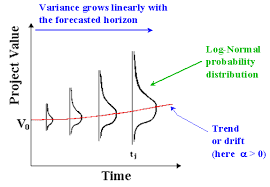
From this graph we can see two things:
-
There is a skew in the price distribution. This is due to the log-normal distribution. Intuitively, there is such skew since prices are floored but not capped. This has the effect to spread more the prices far from zero.
-
The volatility increases with time. This reflects the uncertainty growing with time.
The log-normal density function is:
\[f_X(x) = \frac{1}{x\sigma \sqrt{2 \pi}}\exp\Bigg(-\frac{(\ln(x)-\mu)^2}{2\sigma^2}\Bigg)\]Expected value of $S_t$:
-
$\mathbb{E}[S_t]=S_0e^{\mu t}$ (demo)
-
$\mathbb{E}[S_{t+\Delta t}]=\mathbb{E}[S_{t}]e^{\mu \Delta t}$
Implementation
The below is the implementation of the above formula $(P)$.
# GBM - One path - For loop

mu = .05 # expected return ; needs to be continuous !
n_years = 5
sigma = .2 # should be the same time unit as mu
dt = 0.1 # length of one period ; should be the same time unit as mu
n_periods = int(n_years/dt)
S0 = 100

St = np.zeros(n_periods+1) # +1 to show the starting value S0
St[0] = S0

for t in range(1,n_periods+1):
    St[t] = St[t-1]*np.exp((mu-sigma**2/2)*dt+sigma*np.random.normal(0,1)*np.sqrt(dt))
It is also possible to implement the formula $(P)$ using a vectorized approach (i.e. no for loop) by using the fact that continuous returns are additive:
# GBM - One path - Vectorized

ret = (mu-sigma**2/2)*dt+sigma*np.random.normal(0,1,n)*np.sqrt(dt)
ret_cum = np.cumsum(ret, axis=0) # Note: the cumsum operation is recursive

St = np.exp(ret_cum)
St = np.hstack([1, St])
St = S0 * St
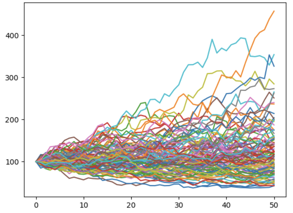
To double check the result, we can generate many paths and average them to match the expected value. This illustrate the concept of Monte Carlo simulations where the objective is to generate random variables many times to estimate a value (expected value):
# GBM - Several paths - For loop

mu = .05
n_years = 5
sigma = .2
dt = 0.1
n_periods = int(n_years/dt)
S0 = 100
n_paths = 100

St = np.zeros((n_paths, n_periods+1))
St[:,0] = S0

for t in range(1,n_periods+1):
    St[:,t] = St[:,t-1]*np.exp((mu-sigma**2/2)*dt+sigma*np.random.normal(0,1,n_paths)*np.sqrt(dt))

print(round(np.mean(St[:,-1]),0) == round(S0*np.exp(mu*n_years),0)) # true with high number of paths

plt.figure()
plt.plot(St.T)
plt.show()