Differential equations

A differential equation is an equation with the following characteristics:

• variables = functions

• it expresses the relationship of functions (variables) with their derivatives

Case of linear and constant coefficient differential equations:

In order to solve such equations, we use characteristic equations. Let $y(x) = e^{rx}$

(E) => $a_nr^n e^{rx} + a_{n-1}r^{(n-1)} e^{rx} + … + a_1 r e^{rx} + a_0e^{rx} = 0$

Since $e^{rx} \neq 0$

(E) => $a_nr^n + a_{n-1}r^{(n-1)} + … + a_1 r + a_0 = 0$

We thus end up with a polynomial function.

In order to find the general solution of (E), we can find the solution of the characteristic equation and deduce the general solution (using exponential).

Autoregressive processes

Autoregressive processes are a specifc case of differential equations.

$y_{t+k} = \beta_1 y_{t+k-1} + \beta_2 y_{t+k-2} + … + \beta_k y_{t}$

Characteristic equation:

$r^k - \beta_1 r^{k-1} - … - \beta_{k-1} r - \beta_k = 0$

Stationary processes

A stationary process has the same moment (expectation, variance, etc.) in every single sample extracted from the main serie. In other words, the distribution of those samples should all be the same.

In practice, we check the stationarity with only the first two moments (expectation and variance).

Intuition behind the importance of stationary processes in regressions:

When performing regressions, it is important to make sure the error term is stationary. If non stationary, there’s probably a trend that is not caught by the explanatory variables used. This can lead to spurious regressions.

To make sure a process is stationary, we have to check the existence of a unit root.

Why existence of unit root leads to non-stationary process?

Toy example:

Let us consider a 1st order autoregressive process $y_t = \beta_0 + \beta_1 y_{t-1} + \epsilon_t$

Let $\beta_0 = 0$. The characteristic equation is:

$r - \beta_1 = 0$

The solution is $r = \beta_1$

The problem has thus a unit root when $\beta_1 = 1$

Since $y_t = \beta_0 + \beta_1 y_{t-1} + \epsilon_t$ we can write:

$y_1 = y_0 + \epsilon_0$

$y_2 = y_1 + \epsilon_1 = y_0 + \epsilon_0 + \epsilon_1$

$y_3 = y_0 + \epsilon_0 + \epsilon_1 + \epsilon_2$

Thus, $y_t = y_0 + \Sigma_{j=0}^t \epsilon_j$

The variance is $\mathbb{V}[y_t] = t \sigma^2$ (we assume a constant variance for $\epsilon$)

Consequently, the variance is increasing with time so the process is not stationary.

To detect stationarity, we can perform a unit root test such as Augmented Dicky Fuller test.

Non stationarity can be corrected in several ways :

• time regression : performing a regression on time and working with the error term

Example : if $y_t$ in non stationary

$y_t = \beta_0 + \beta_1 t +\epsilon_t$ –> $\epsilon_t$ will not depend on time anymore

• finite differences : removing previous term to each observation $y_t = y_t - y_{t-1}$ –> this will have the effect to remove the trend

• moving average NxN

Example : using (double) centered moving average 5x5.

cpi_roll = cpi.rolling(window=5).mean() # cell at index 4 is the mean of the 5 previous ones (inclusive)
cpi_mm = cpi - cpi_roll
cpi_roll_2 = cpi_mm.rolling(window=5).mean()
cpi_mm_2 = cpi_mm - cpi_roll_2

Example: using exponential moving average.

When averaging over an infinite number of values, we can write:

Weights are decreasing exponentially. Indeed, the weights are $(1-\alpha)^n$ and since $1-\alpha < 0$, the weights decrease when raised with a power. Below is the plot of the weights against the observations’ indexes (the lowest index is the most recent):

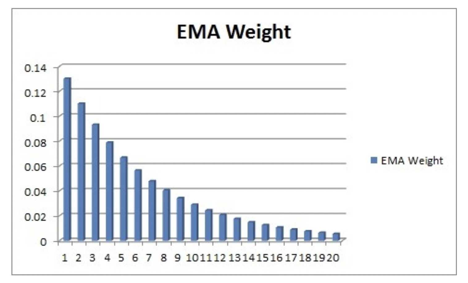
We also have the relationship: $\alpha = \frac{2}{span + 1}$ where span is the number of periods to be using in the computation.