The PCA’s objective is to get an approximation of data in a low dimensional space.

Inertia

Inertia $I_M = \Sigma_{i=1}^n p_i ||x_i - g||_M^2$

Note: the inertia in physics is equivalent to the variance in statistics

where $g^T = (\bar{x}^{(1)},…,\bar{x}^{(p)})$ also called the gravity center.

–> The inertia is thus the weighted average of the squared distance of each observation with the gravity center.

–> $p_i$ is the weight given to each observation. Most of the times, $p_i = \frac{1}{n}$ (every observation contributes equally to the analysis)

–> the distance $||.||$ depends on the choosen metric $M$

If the data are centered:

Since $I_M \in \mathbb{R}$:

Thanks to the trace properties:

With $V = Cov(X)$:

Projection

In order to represent the data in a low dimensional space, we use projections.

The projection should distort the initial space the less as possible, that is:

=> reduce the projection distances as much as possible

=> maximize the average of squared distances between projected points

=> maximize inertia of the projected points

In the below figure, maximizing the inertia leads to choosing the projection on the right since d2 > d1.

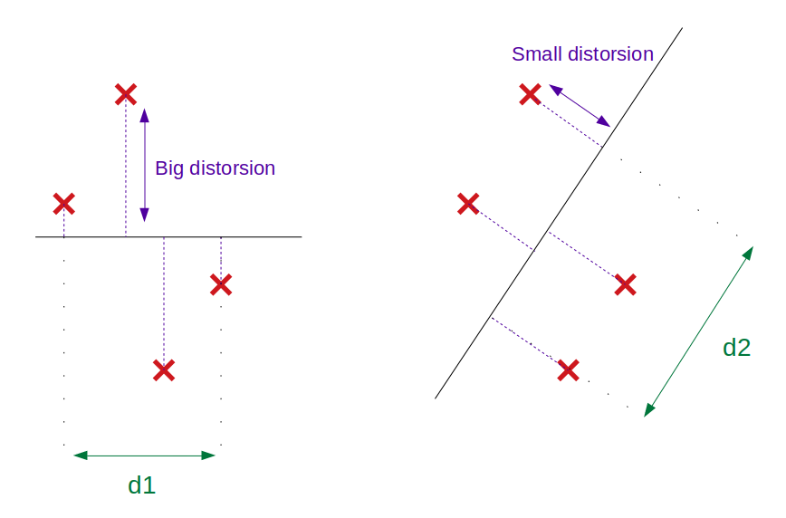
The above figure shows that PCA achieves a dual objective: finding the maximum variance of the projected space (green arrow = projected variance) as well as minimizing the squared distance from projected space to the initial data (blue arrow). In that sense, PCA is also often described as a form of OLS.

Let $P$ a projector. $V = Cov(X) = X^TDX$ (with $D$ the weight matrix). The covariance matrix of the projected points is:

Note: a projector $P$ is such that $P^2=P$ and $PM = MP^T$

Optimisation

As seen previously, the objective is to maximize the inertia. Combining the previous 2 paragraphs, we can express the inertia of projected points:

$Tr(PVP^TM) = Tr(PVMP)$ since $PM = MP^T$

$~~~~~~~~~~~~~~~~~~~~~~~~= Tr(VMP^2)$ since $Tr(AB) = Tr(BA)$

$~~~~~~~~~~~~~~~~~~~~~~~~= Tr(VMP)$ since $P^2 = P$

Thus the optimisation problem is:

The objective is to find the line (in black on above figure) going through $g$ and maximizing the inertia. Let $a$ be a point on this line. We have the following equation:

(Indeed we have $P^2=P$ and $PM = MP^T$)

$Tr(VMP) = Tr(VMa(a’Ma)^{-1}a’M)$

$~~~~~~~~~~~~~~~~~~= \frac{1}{a’Ma}Tr(VMaa’M)$

$~~~~~~~~~~~~~~~~~~= \frac{Tr(a’MVMa)}{a’Ma}$

$~~~~~~~~~~~~~~~~~~= \frac{a’MVMa}{a’Ma}$ since $a’MVMa$ is a scalar

In order to obtain the maximum, we use first order optimal conditions:

With $\frac{d}{da}(\frac{a’MVMa}{a’Ma}) = \frac{(a’Ma)2MVMa-(a’MVMa)2Ma}{(a’Ma)^2}$, previous equation becomes:

$MVMa = (\frac{a’MVMa}{a’Ma})Ma$

Since $\frac{a’MVMa}{a’Ma}$ is a scalar, let’s replace it by $\lambda$:

Based on eigenvalue definition, $\lambda$ is thus the eigenvalue of $VM$.

We can thus rewrite the optimization problem:

This final result leads to the theorem:

The lower dimensional space is given by the eigenvectors associated with the biggest eigenvalues.

Summary of the proof:

Minimization of the distorsion => maximization of the inertia of the projected space => maximization of the covariance matrix’s eigenvalues.

In practice, we simply use the Spectral Decomposition of the covariance matrix:

where $U$ is a matrix with eigenvectors in column. $D$ is the new covariance matrix in the orthogonal (all covariances are zero) projected space. The eigenvectors represent the main directions of the variability of the reduced space, whereas the eigenvalues represent the magnitudes for the directions. See more details in a step-by-step example here.

Implementation

import numpy as np

def PCA(X , num_components):
 
    # Standardize variables
    X_std = (X - np.mean(X))/np.std(X)
 
    # Compute covariance matrix
    cov_mat = np.cov(X_std , rowvar = False)
 
    # Find eigenvalues and eigenvectors (results of a matrix decomposition)
    eigen_values, eigen_vectors = np.linalg.eig(cov_mat)
    # Reminder: cov_mat == eigen_vectors @ np.diag(eigen_values) @ eigen_vectors.T
    
    # Sort eigenvalues and eigenvectors
    sorted_index = np.argsort(eigen_values)[::-1]
    sorted_eigenvalue = eigen_values[sorted_index]
    sorted_eigenvectors = eigen_vectors[:,sorted_index]
    
    # Keep eigenvectors associated with highest eigenvalues
    eigenvector_subset = sorted_eigenvectors[:,0:num_components]
    
    # Compute the reduced space
    X_reduced = X_std @ eigenvector_subset
    # X_reduced is the projection of the initial dataset    
    # eigenvector_subset is the projector
    
    return X_reduced

Note (1): standardizing is a good practice before PCA; if not done, variables with high variances will have too much importance. Useful details here and here.

Explanation of the components

The principal components are a result of a matrix multiplication. Consequently, the principal components can be written as linear combinations of the initial features:

def explain_pca(eigenvector_subset, feature_names=[]):
    dict_res = {}
    weight_list =[[] for i in np.zeros(eigenvector_subset.shape[1])]
    if feature_names == []:
        feature_names = ['feat ' + str(i) for i in range(eigenvector_subset.shape[0])]
    for idx_col in range(eigenvector_subset.shape[1]):
        pc_str = 'PC' + str(idx_col+1)
        sum_col = np.sum(abs(eigenvector_subset[:,idx_col]))
        for idx_row in range(eigenvector_subset.shape[0]):
            weight = round(eigenvector_subset[idx_row, idx_col]/sum_col, 2)
            new_explanation = '{} = {}'.format(feature_names[idx_row], weight)
            if pc_str in dict_res:
                dict_res[pc_str].append(new_explanation)
            else:
                dict_res[pc_str] = [new_explanation]
            weight_list[idx_col].append(weight)
    return dict_res, weight_list