1) Accuracy

The accuracy is the percentage of correct predictions:

where $\hat y$ is the prediction and $y$ the true value.

Note: for imbalanced data, the accuracy can be very misleading because a classifier can achieve a high score just by predicting the majority class with probability 1.

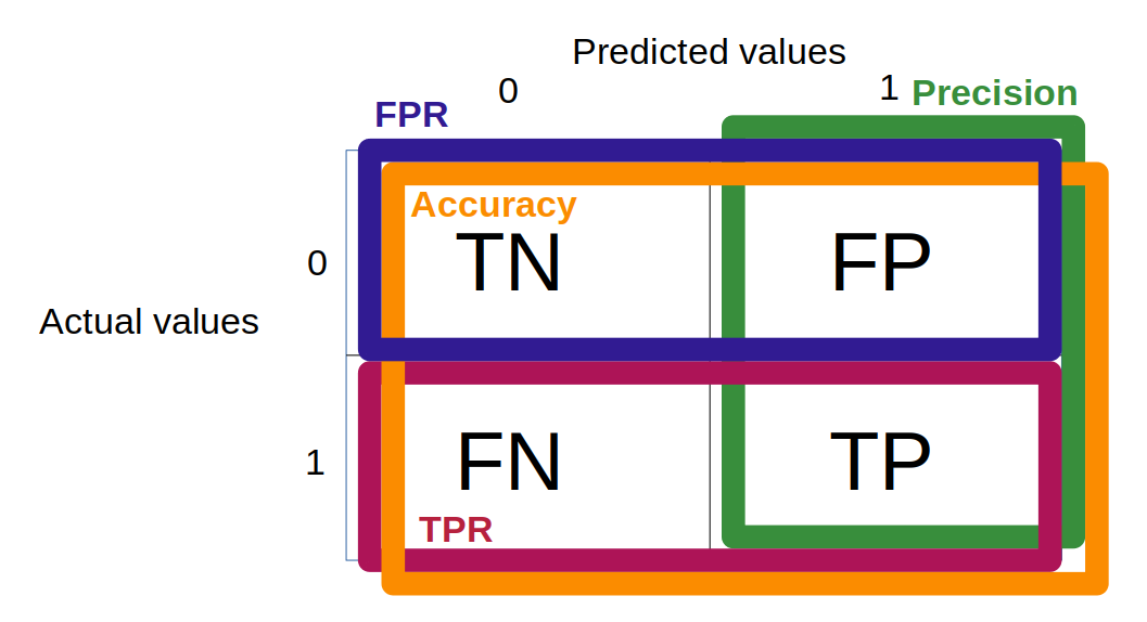
In case of binary classification, the accuracy can be written as such: $accuracy = \frac{TP + TN}{TP + TN + FP + FN}$

2) True positive rate

The TPR measures the proportions of positives that are correctly identified.

Note: this metric is typically used for medical tasks as it is crucial to minimize the count of false-negatives.

3) False positive rate

The FPR measures the proportions of negatives that are correctly identified.

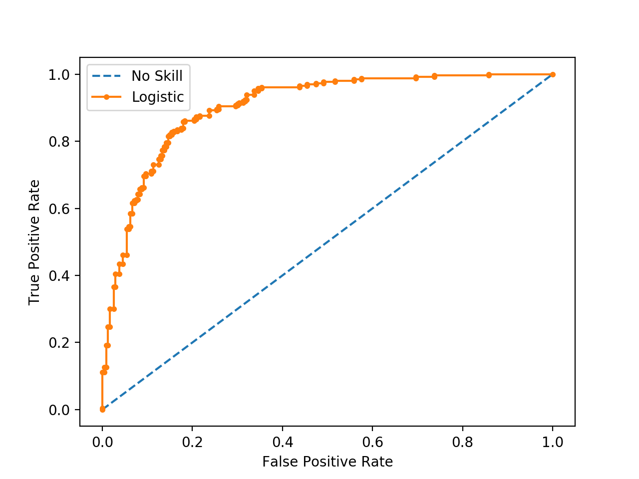
4) ROC (Receiver Operating Characteristic) curve

The ROC curve combines the $TPR$ and $FPR$.

Use of the ROC

If one model is used:

We use the ROC curve to evaluate the performance of one classifying model that we can obtain when varying a threshold.

If several models are used:

We use the ROC curve to compare several classifiers in evaluating the area under the curve (AUC) for a range of thresholds.

Intuition

After running the prediction of a specific model, we draw the confusion matrix (see below) with a certain threshold.

We then modify the threshold and draw another confusion matrix.

The ROC curve summarizes all of the confusion matrices that each threshold produced.

Implementation

1. Get probability predictions

2. Sort the probabilities (prediction)

3. Sort the validation (actual) according to previous sort

4. Loop on the sorted validation. At each iteration:

• increment TP or FP

• compute the TPR and FPR.

1. Plot (FPR, TPR)

See this link for an implementation example. Below is also a computation of TPR from ChatGPT to better understand the relationship between thresholds and TPR:

prob = clf.predict_proba(X_test)
prob_pos = prob[:,1] # probabilities for the positive class
fpr, tpr, thresholds = metrics.roc_curve(y_test, prob_pos, pos_label=1)

recomputed_tpr = []

# Iterate through each threshold
for threshold in thresholds:
    # Use the current threshold to determine the predicted labels based on probabilities
    predicted_labels = np.where(prob_pos >= threshold, 1, 0)
    
    # Calculate True Positives (TP), False Negatives (FN), False Positives (FP), and True Negatives (TN)
    TP = np.sum((predicted_labels == 1) & (y_test == 1))
    FN = np.sum((predicted_labels == 0) & (y_test == 1))
    
    # Calculate True Positive Rate (TPR) for the current threshold
    current_tpr = TP / (TP + FN) if (TP + FN) > 0 else 0.0
    
    # Append the TPR value to the list
    recomputed_tpr.append(current_tpr)

5) Precision

Note: this metric should be used when false-negative is not too much a concern (e.g. YouTube recommendations, trading strategies). It can also be used when the data are imbalanced (see details below).

6) PR (Precision Recall) curve

The PR curve combines $TPR$ (recall) and $precision$.

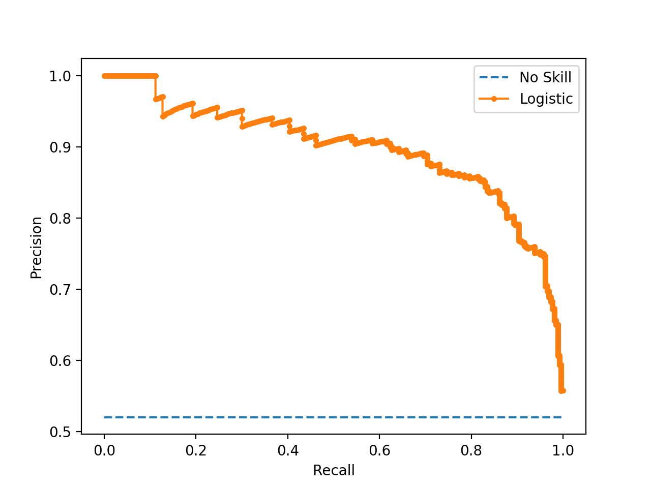
The PR curve is better adapted than the ROC curve in the case of imbalanced data:

ROC curve uses $FPR = \frac{FP}{\color{red}{N}} $ –> $N$ can be either very large or very small if classes are imbalanced.

PR curve uses $\text{Precision} = \frac{TP}{\color{green}{TP + FP}}$ –> the precision considers only the positive values coming from the model.

7) F1-score

F1-score is a single metric that combines TPR (recall) and precision.

Note: it is widely used for imbalanced datasets since it involves the precision.

Metric summary