A test is parametric if its goal is to test parameters of a known/unknown distribution.

Note: we call population the total data from which a sample is extracted. A statistical test aims at finding information about the distribution the sample is extracted from.

Procedure:

1) find the test to perform

2) find the right estimator to use

3) deduce the reject region

4) compute the test statistic

5) retrieve quantiles of known distributions

See the associated notebook for numerical examples.

Example 1 (Z-test):

$X_1,…,X_n~(iid)\sim \mathbb{P_\theta}$

We want to know the mean of an unknown distribution from which we have a sample.

Requirements/assumptions:

• we need the population to be normally distributed. Note: this may not be needed when sample size is high (> 30) as CLT will anyway give normality

• we need the standard deviation of the population

1) find the test to perform

2) find the right estimator to use

Since we are testing the mean, we choose the empirical mean as estimator $\widehat{\theta}=\frac{1}{n}\sum{X_i}$

3) deduce the reject region

We fix $k$ for a rejection level $\alpha$. The rejection region is \(Z= \{\widehat{\theta} \ge k\}\)

We look for $k$ defined as such:

$\mathbb{P}_{\theta \in \Theta_0}(\widehat{\theta} \ge k)=\alpha$ => under $\mathcal{H}_0$, we reject the hypothesis when our estimator $\widehat{\theta}$ is above $k$

Intuitively, we want to keep our hypothesis if it’s verified in most of the cases => under our hypothesis, there is a low probability that we are in the rejection region.

Thus, if in real life we have a result that makes the hypothesis unverified, we reject the hypothesis. However, we have a risk of $\alpha$ that our hypothesis was correct and that we ended up in the rejection region by mistake.

4) compute the test statistic

We center and reduce the estimator in order to get the Gaussian law and thus end up with known quantiles:

\(\mathbb{P}_{\theta = a}(T \ge \frac{\sqrt{n} (k-a)}{\sqrt{\sigma^2}})=\alpha\) with $T \sim_{n \to \infty} \mathcal{N}(0,1)$

$T$ is the test statistic (a test statistic is a random variable for which we know the law under $\mathcal{H}_0$)

5) retrieve quantiles of known distributions

Finally, $\frac{\sqrt{n} (k-a)}{\sqrt{\sigma^2}}=q_\alpha$ => we can find $k$ telling us when rejecting $\mathcal{H}_0$

Why not looking at the average directly?

=> the average can be influenced by the outliers and thus doesn’t take into consideration extreme events.

How about the median?

=> the median doesn’t take into account the distribution / tendency of the values.

The p-value is the lowest error probability we want to make when rejecting our hypothesis.

The lower the p-value is, the less error we make in rejecting our hypothesis so the more significant the rejection is.

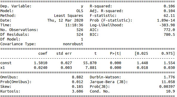
When performing OLS, our hypothesis is $\theta_{x1}=0$ so we don’t reject it if the pvalue column is higher than our threshold. In the below OLS result, pvalues are displayed in column $P>|t|$. All variables are significant.

Example 2 (T-test): when the variance is not known.

Say we want to test whether a coefficient is zero:

1) find the test to perform

2) find the right estimator to use

$\widehat{\theta_j} = (X^TX)^{-1}X^TY$

3) deduce the reject region

$Z={k_1 \leq \widehat{\theta_j} \leq k_2}$

4) compute the test statistic

$T_j = \frac{\widehat{\theta_j}-\theta_j}{\sigma_{\theta_j}} = \frac{\widehat{\theta_j}}{\sigma_{\theta_j}} \sim \mathcal{N}(0,1)$ with $\sigma_{\theta_j} = \sigma \sqrt{(X^TX)^{-1}}$ (recall that $\sigma = \sigma_{\epsilon}$)

Since we don’t know $\sigma$, we can use the Cochrane theorem to remove this value:

$T_j = \frac{ \frac{\widehat{\theta_j}}{\sigma \sqrt{(X^TX)^{-1}}} \sim \mathcal{N}(0,1)}{\sqrt{\frac{\widehat{\sigma}^2 (n-p-1)}{\sigma^2} \sim \mathcal{X}_{n-p-1}}} \sim \mathcal{T}(n-p-1)$ with $\widehat{\sigma}^2 = \frac{1}{n-p-1} \Sigma \epsilon ^2$

$T_j = \frac{\widehat{\theta_j}}{\Sigma \epsilon ^2 \sqrt{(X^TX)^{-1}}}$

5) retrieve quantiles of known distributions

Finally,

$\mathcal{P}_{\theta_j=0}(\frac{k_1}{\Sigma \epsilon ^2 \sqrt{(X^TX)^{-1}}} \leq T_j \leq \frac{k_2}{\Sigma \epsilon ^2 \sqrt{(X^TX)^{-1}}}) = \alpha$

Thus, $\frac{k_1}{\Sigma \epsilon ^2 \sqrt{(X^TX)^{-1}}} = t_{\frac{\alpha}{2}}$ (same for $k_2$)

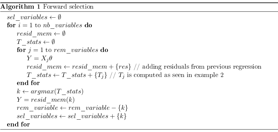
Example 3 (T-test with forward selection):

Concept: regress all variables one by one on the most significant variable’s residual, remove the most significant variable after each full round.

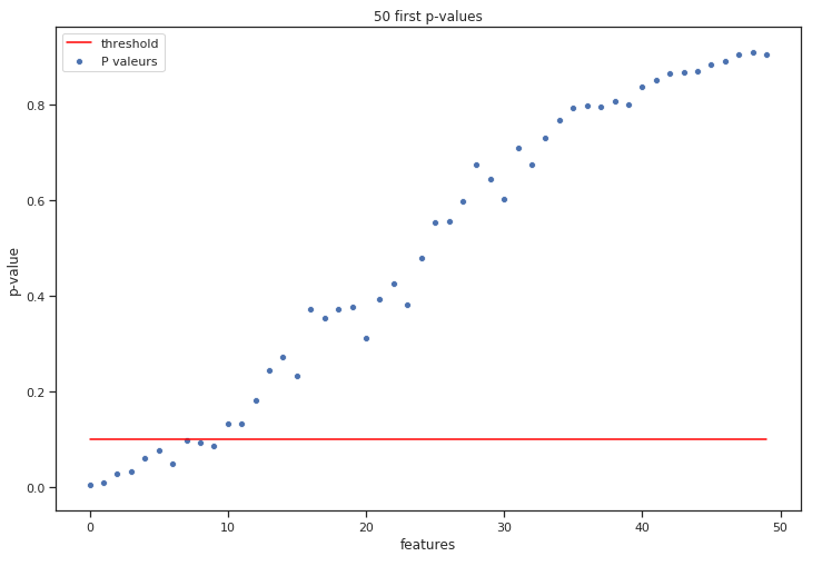
(x-axis is the order in which we selected variables)

We can then select only the most significant variables based on p-values on variables from list \(sel\_variables\)

Note: since \(pval = 2*(1-cdf(T)) = 2*\frac{1-(1-\alpha)}{2}\), choosing the biggest T-stat is equivalent to choose the smallest p-value

Example 4 (F-test):

When several variables are correlated (often the case in practice), the student test is not efficient enough since it does not take the correlation into account. F-test allows to test global significativity.

Let’s say we have 4 variables and we want to check the significativity of 2 of them.

$SSR = sum~squared~residuals = \Sigma (\widehat{y_i} - y_i)^2$

$F = \frac{(SSR_C - SSR_{NC})/(p_{NC} - p_C)}{(SSR_{NC})/(n-p_{NC})} \sim \mathcal{F}(p_{NC} - p_C, n-p_{NC})$

NC: not constraint model

C: constraint model

Method:

• OLS on not constraint model => computation of $SSR_{NC}$

• OLS on constraint model => computation of $SSR_{C}$

• Computation of the Fisher stat => computation of p-value (using complementary cdf as above)

# Non constraint model
X0=np.column_stack((educ, exper, tenure, const))
model=sm.OLS(y,X0)
results = model.fit()
u=results.resid
SSR0=u.T@u

# Constraint model
X=np.column_stack((const, educ, tenure))
model=sm.OLS(y,X)
results = model.fit()
u=results.resid
SSR1=u.T@u

# Computation of Fisher stat
n=np.shape(X0)[0]
F=((SSR1-SSR0)/1)/(SSR0/(n-4))
f.sf(F,1,n-4) # p-value

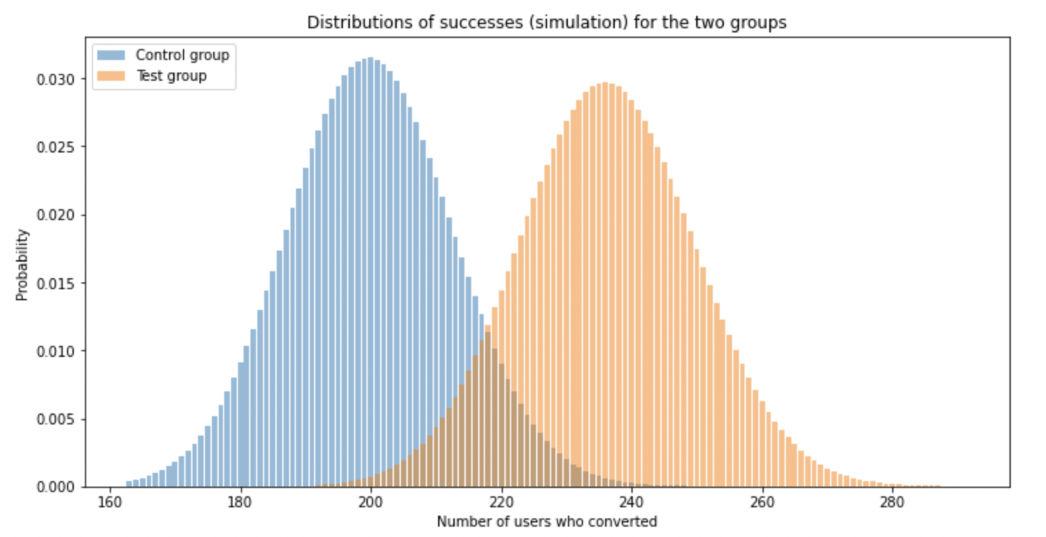
Example 5 (AB-test):

A/B tests are typically used in digital marketing. Two groups of people are randomly selected:

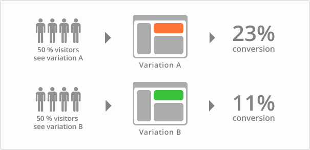
People in group A (control group) see version A and people in group B (test group) see version B. The assessed metric is the conversion rate i.e. the proportion of users who clicked on the “Buy” button.

We can define two random variables $X_A$ and $X_B$ to modelize the clicks. Those variables are binary: 0 (no click) or 1 (click).

If we repeat the experiment many times (with different samples), the two variables follow a Binomial distribution:

Below is an example of results following the experiment:

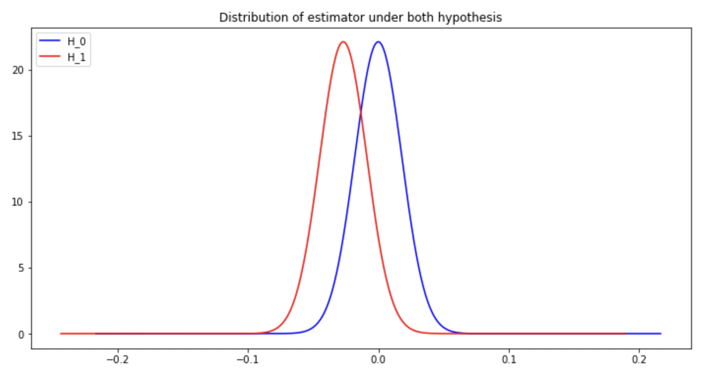
The two hypothesis are:

Where $p_A$, $p_B$ are the true conversion rates.

Since the variables are binary, we can estimate the conversion rates with the empirical mean:

Our final estimator (according to $\mathcal{H}_0$) is thus $\hat p_A-\hat p_B$. Thanks to the CLT,

Thus,

Note: $p_A$ and $p_B$ in the variance are not known. We may use estimated values (to be verified).

We can now plot the estimator under both hypothesis:

Significance level: probability of false positives i.e. the probability of wrongly rejecting the null hypothesis. Using $\alpha$ as a significance level, $\mathbb{P}_{\mathcal{H}_0}(\hat d >k)= \alpha/2$.

Thus $k = q_{1-\frac{\alpha}{2}}\sigma_{\hat d} + 0$. We can deduce the confidence interval $[-q_{1-\frac{\alpha}{2}}\sigma_{\hat d}, q_{1-\frac{\alpha}{2}}\sigma_{\hat d}]$

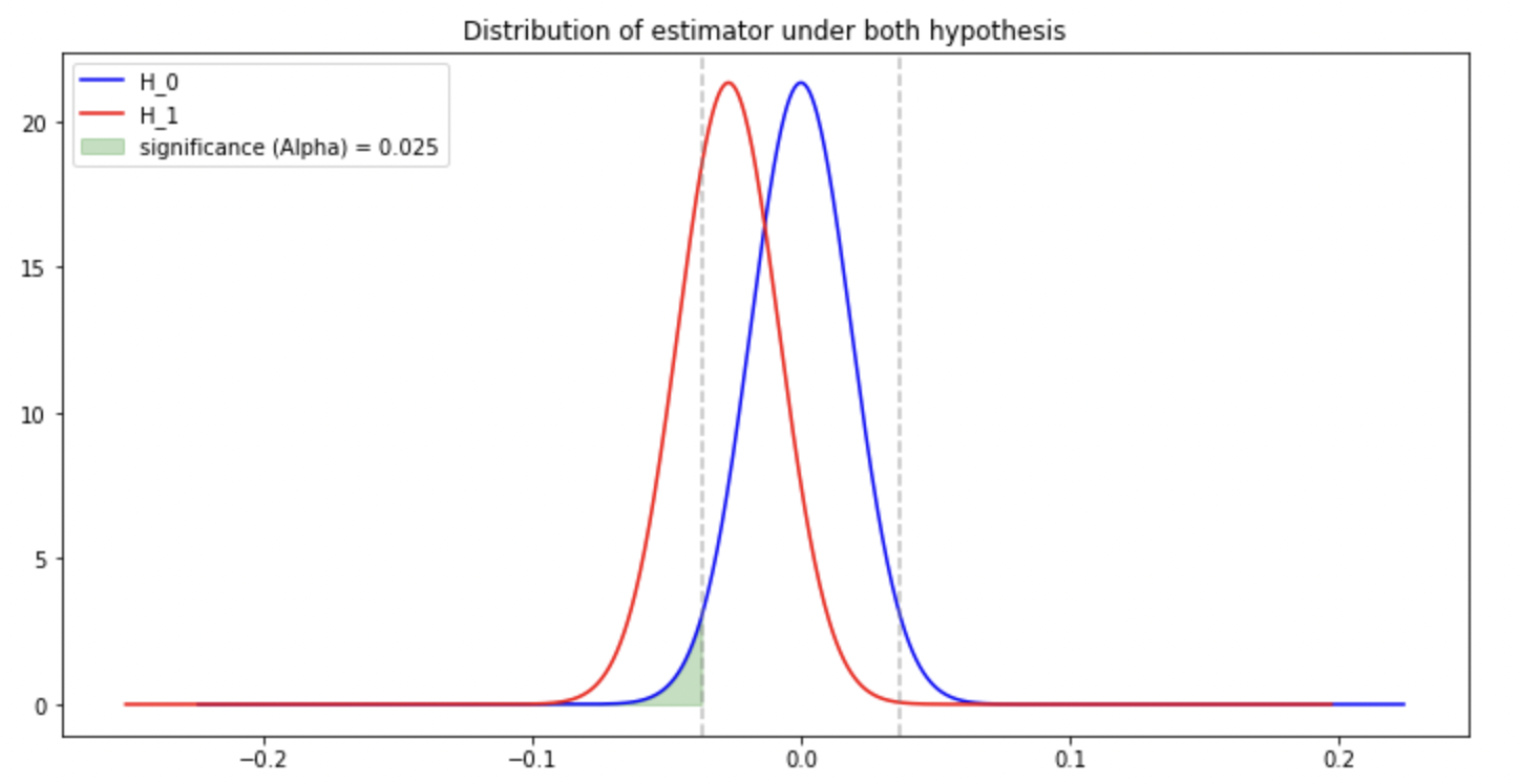
Power of the test: probability of true positive i.e. the probability of correctly rejecting the null hypothesis. Intuitively, the more the two shapes are separated, the more true positives we have.

Note: increasing the number of observations has the effect of reducing the standard deviation of both estimators ($\mathcal{H}_0$ and $\mathcal{H}_1$) and thus add more space between the two shapes => increase the power of the test.

Example 6 (Z-test (other explanation)):

Procedure:

1) Define the test to perform

2) Find the right estimator to use

3) Bring the estimator to a known distribution

4) See how likely is our real-life example based on the known distribution

1) Define the test to perform.

2) Find the right estimator to use. Since we are testing the mean, we choose the empirical mean as estimator $\widehat{\theta}=\frac{1}{n}\sum{X_i}$

3) Bring the estimator to a known distribution. Thanks to CLT, we know that the estimator follows a normal distribution.

In particular, under $\mathcal{H}_0$, $\widehat{\theta} \sim \mathcal{N}(a, \frac{\sigma}{\sqrt{n}})$ where $\sigma$ is the standard deviation on the population (known).

3) See how likely is our real-life example based on the known distribution.

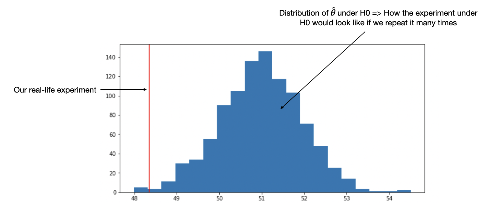
We can see that the result we got “in real life” is very unlikely to happen if we repeat the experiment under $\mathcal{H}_0$ many times. Thus, we can reject $\mathcal{H}_0$. However, there’s still a chance (<5%) that $\mathcal{H}_0$ is true and that our real life example is just an extreme event.

Example 7 (Z-test (proportions)):

(i) We believe there are the same number of women than men in the population. Our sample has $n=100$ people including $k=45$ females. Is our sample representative enough?

(ii) We toss a coin $n=50$ times and get $k=30$ heads. Is the coin fair?

1) Define the test to perform. $\mathcal{H}_0: p=p_0$

2) Find the right estimator to use. \(\hat p = \frac{n_{success}}{n}\)

3) Bring the estimator to a known distribution. $X \sim \mathcal{B}(n,p)$ with $X$ the number of successes. Thanks to normal approximation, we have (under $\mathcal{H}_0$):

$X \sim \mathcal{N}(np_0, \sqrt{np_0(1-p_0)})$ with $X$ the number of successes.

Thus: $\hat p \sim \mathcal{N}(p_0, \sqrt{\frac{p_0(1-p_0)}{n}})$

4) See how likely is our real-life example based on the known distribution (illustration of example (i) above).

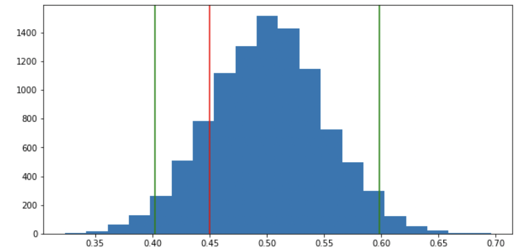
We can see that the result we got “in real life” is likely to happen if we repeat the experiment under $\mathcal{H}_0$ many times. Thus, we can’t reject $\mathcal{H}_0$.

The rejection region is outside the confidence interval. For a level of $95\%$, we don’t reject $\mathcal{H}_0$ if $\hat p \in [p_0 \pm 1.96 \sqrt{\frac{p_0(1-p_0)}{n}}]$.

Note: if $n$ is too small, the normal approximation is not accurate enough. One can use the binomial test instead (if $p_0 \neq 0.5$ the easiest way is to use “Equal distance from expected” described here). Another option is to use an “abaque” as explained here. See example 8 for an illustration on a toy example.

Notes about confidence intervals:

• a confidence interval is always around an estimator.

• the size of the confidence interval decreases with the number of observations. Intuitively, when dealing with a lower number of observations, we need to have more extreme results to safely reject $\mathcal{H}_0$.

Example 8 (Binomial test):

(i) My trading strategy placed 4 trades, all successful. Can I say that my results are statistically significant?

(ii) I met 4 French people, they were all arrogant. Can I deduce that all French people are arrogant?

1) Define the test to perform: $\mathcal{H}_0: p=50\%$ where $p$ is the true proportion of trades that were successful.

2) Find the right estimator to use: $\hat p = \frac{n_{success}}{n}$.

3) Bring the estimator to a known distribution: $\hat p \sim \mathcal{B}(n,p)$.

4) See how likely is our real-life example based on the known distribution. Using the binomial pdf: $\mathbb{P}_{\mathcal{H}_0}(X=4) = C_4^4(50\%)^4(1-50\%)^{4-4} = (50\%)^4 = 6.25\%$

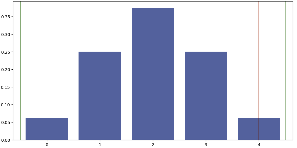
Even though the success rate is very high, the distribution doesn’t allow to safely reject the null hypothesis.

Moreover, the power of the test is rather low (because of small sample size). E.g. if we assume the true success rate is 80%, the two curves are highly overlapping each other.

import scipy.stats as scs

fig, ax = plt.subplots(figsize=(12,6))
n = 4
p = 0.5

# null hypothesis
x = np.arange(0, n+1)
y_null = scs.binom(n, p).pmf(x)
ax.bar(x, y_null, alpha=0.5, label='estimator under H_0')

# alternative hypothesis
y_alt = scs.binom(n, 0.8).pmf(x)
ax.bar(x, y_alt, alpha=0.5, label='estimator under H_1')

# critical values
# dist = scs.binom(n, p)
# critical_value = dist.ppf(.95)
# ax.axvline(x=4.5, c='green', alpha=0.5, linestyle='-')
# ax.axvline(x=-0.5, c='green', alpha=0.5, linestyle='-')
# ax.axvline(x=4, c='red', alpha=0.5, linestyle='-')

# overlapping area
overlap = np.minimum(y_null, y_alt)
overlap_area = round(np.sum(overlap),1)
ax.bar(x, overlap, alpha=0.5, color='purple', label='Overlap={} (power={}%)'.format(overlap_area,round((1-overlap_area)*100)))