Assumptions
Preamble: errors are the deviations of the observations from the population, while residuals are the deviations of the observations from the sample.
$Y^{population}_i = \alpha + \beta X^{population}_i + \epsilon_i$ –> $\epsilon_i$ are the errors.
$\hat Y^{sample}_i = \hat \alpha + \hat \beta X^{sample}_i + \hat \epsilon_i$ –> $\hat \epsilon_i$ are the residuals.
The assumptions behind the classical linear regression (OLS - Ordinary Least Squares) model are:
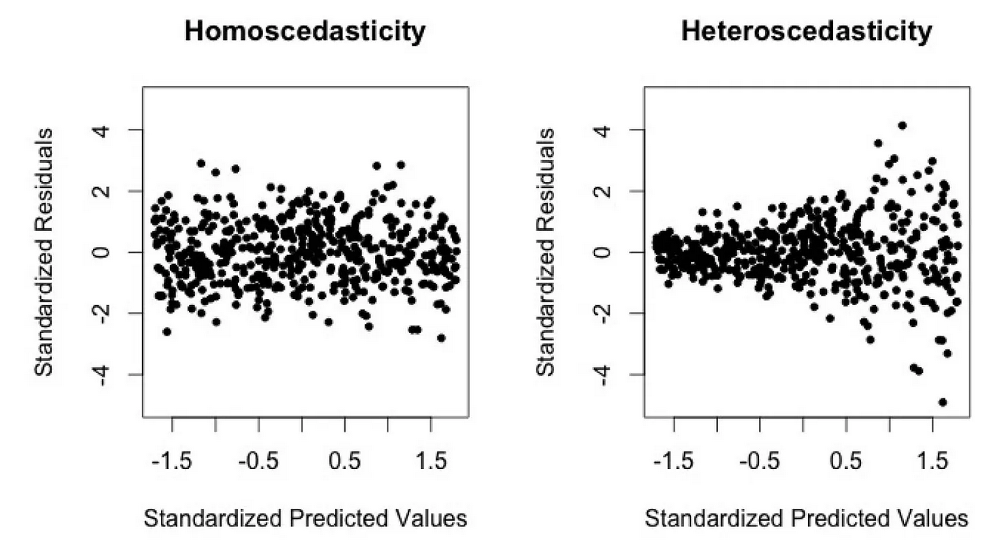
- The variance of errors is constant (homoscedasticity): $\mathbb{V}[\epsilon] = \sigma$.
In other words, the model is “equally good” no matter how low/high are the values of the predictor. Example: say we predict stock prices based on market capitalization. Heteroscedasticity would be if the residuals get larger with the market capitalization meaning that the model would be increasingly bad when dealing with larger companies.
Without homoscedasticity, the estimator becomes unstable (high variance i.e. very sensitive to data). To identify homoscedasticity, one can plot the residuals against the predicted values; if there is a trend, then homoscedasticity may be violated. Another possibility is to run through statistical tests such as the White test.
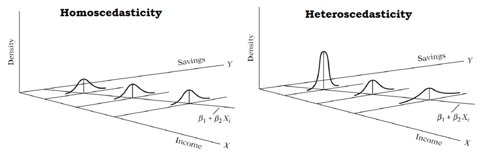
Note (1): plotting the dependent variable against the independent variable can also give a hint on whether to expect heteroscedasticity or not (see picture below). However this method is less generic as it focuses on one predictor only.
Note (2): homoscedasticity doesn’t say anything about the correlation between predictors, nor between errors, nor between errors and predictors.
- The errors have conditional mean of zero (exogeneity): $\mathbb{E}[\epsilon | X] = 0$.
If there is no exogeneity, then the estimator is biased.
Case 1: omitted variable
A typical example is $Y = \beta_0 + \beta_1 X + \epsilon$ where: Y = ice cream sales; X = swimming suit sales; C (omitted) = weather. In this regression, X is not exogenous in the sense that it also depends on other (omitted) variables such as the weather. The omitted variable is called confounding variable.
In such case, the error (and not the residuals) will be highly correlated to the predictor since it contains the omitted variable (weather). $\epsilon = Y-(\beta_0+\beta_1 X)$ (note: $\beta_0$ and $\beta_1$ are the true coefficients) -> the error contains the influence of the weather => the error is correlated with X. Hence $\mathbb{E}[\epsilon | X] \neq 0$. Also, $\hat \beta_1$ is likely to be overestimated since it also integrates the weather, leading to a bias.
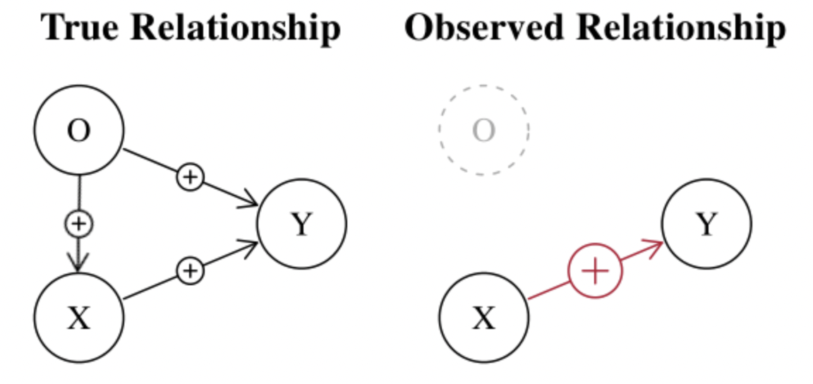
a) Strong under/overestimation
If both X and O impacts positively (resp. negatively) Y, then $\hat \beta_1$ will be overestimated (resp. underestimated) because it includes the effect of the 2 variables.
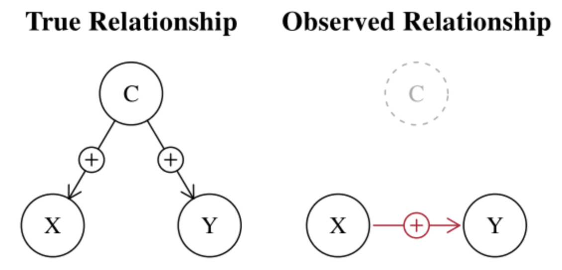
b) Spurrious relationship
The ice-cream example is a typical example of spurious correlations i.e. finding cause when there is actually none.
Another typical example is illustrated by a common mistake many people do when predicting market moves using prices instead of returns. Prices are often non stationary (i.e. they have a trend), hence the best prediction of tomorrow’s price is today’s price. The reason is that prices follow a highly autocorrelated process (they change incrementally rather than jumping unpredictably). This can lead to artificially high correlation between today’s price and tomorrow’s price => spurious relationship.
c) Hidden relationship
The omitted variable can also hide the relationship:
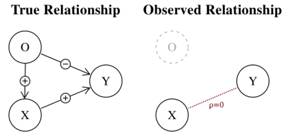
An intuitive example in the financial context of omitted variables is the famous Fama-French model $r = R_f + \hat \beta_1 (R_m - R_f) + \hat \beta_2 SMB + \hat \beta_3 HML + \hat \epsilon$ where:
-
$SMB$ = Small Minus Big (market capitalization)
-
$HML$ = High Minus Low (book-to-market)
It’s obvious that many factors are missing in this simple model (e.g. liquidity, market news, etc.)
Case 2: reverse causality
Reverse causality occurs when $X$ is caused by $Y$. Say the true relationship is $Y = \beta_0 + \beta_1 X + \epsilon$ however we wrongly identify the relationship and work with the model $X = \alpha_0 + \alpha_1 Y + \eta$.
This leads to $X = \alpha_0 + \alpha_1 (\beta_0 + \beta_1 X + \epsilon) + \eta => X = \frac{\alpha_0 + \alpha_1 \beta_0 + \alpha_1 \epsilon + \eta}{1-\alpha_1 \beta_1}$. Here, $X$ depends on $\epsilon$, which violates the assumption that $X$ and $\epsilon$ are uncorrelated.
An intuitive example in the financial context of reverse causality is when trying to predict a stock price using the volatility:
-
high volatility can attract more investors to buy/sell, hence impacting the price
-
low prices can lead to a strong sell off, hence increasing the volatility
To test for exogeneity, one can try out several combinations of independent variables. If the coefficients change, there is an omitted variable. However, often times all variables are not known. Hence there are no real tests for exogeneity. It’s more based on qualitative tests i.e. one would need to think if Y is really caused solely by X.
Note: checking $\frac{1}{n} \sum \hat \epsilon_i = 0$ is not sufficient, this just makes sure the regression line is the best we could draw with the given data.
In practice, exogeneity is almost always violated. Especially when predicting a stock price, it’s impossible to include all variables that are involved in determining the price.
- The errors are uncorrelated $\mathbb{E}[\epsilon_i \epsilon_j] = 0$.
When errors are autocorrelated, the estimator is still unbiased but not with minimal variance. The tests to detect autocorrelation of errors are Durbin-Watson or Ljung-Box. To correct for this problem, one would need to try to include other variables or do some transformations (see $AR(k)$ processes).
Additional assumptions are also sometimes necessary:
-
The explanatory variables are linearly independent. In other words, this means that the matrix $X$ has full rank. If this is not the case, the variance becomes unstable (see “Bias and variance-covariance” section below).
-
The errors are normally distributed.
If the first three assumptions are satisfied, under the Gauss-Markov theorem the OLS estimator is said BLUE (Best Linear Unbiased Estimator). It is unbiased and is has the lowest variance. When the assumptions are violated, it may be better to use the Generalized Least Squares (GLS) or the Weighted Least Squares (WLS) which is a special case of the GLS.
\[\widehat \theta_{OLS} = (X^TX)^{-1}X^TY\] \[\widehat \theta_{GLS} = (X^T\Omega_\epsilon^{-1}X)^{-1}X^T\Omega_\epsilon^{-1}Y\] \[\text{where } \Omega_\epsilon = \mathbb{E}[\epsilon_i \epsilon_j] \text{ i.e. the matrix variance-covariance of the errors}\]Note: LinearRegression from scikit-learn does OLS.
Example: see associated notebook for numerical examples.
R2
\[R^2 = 1-\frac{\sum (y_i - \hat y_i)^2}{\sum (y_i - \overline y)^2}\]Or:
\[R^2 = \frac{\sum (y_i - \overline y)^2 - \sum (y_i - \hat y_i)^2}{\sum (y_i - \overline y)^2} = \frac{\text{variance explained by the regression}}{\text{variance of }y}\]Problems with $R2$:
- $R2$ tends to drop when the variance is high. However, even if the variance is high, there can still be a strong linear relationship between the data.
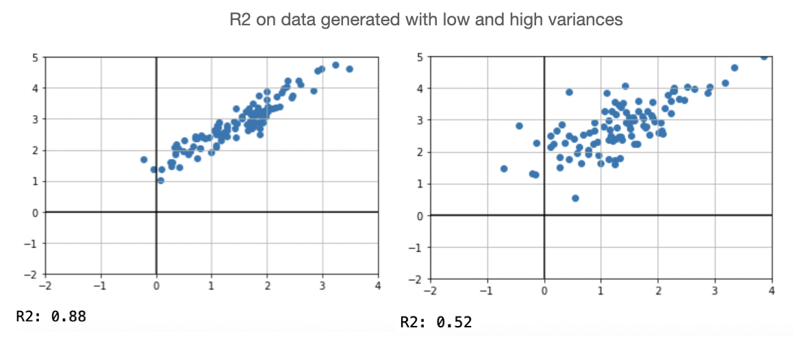
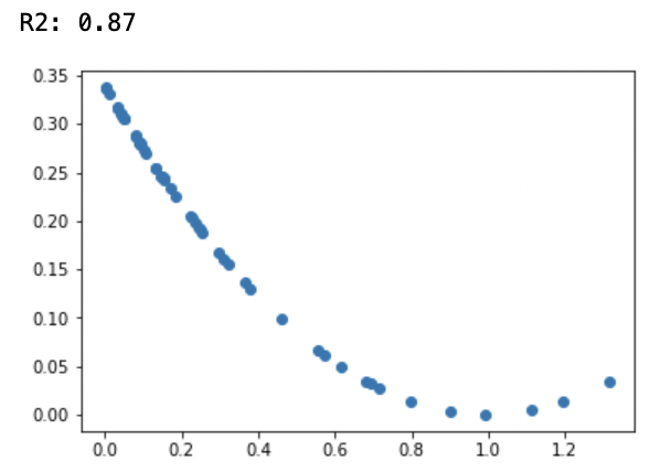
- More generally, high $R2$ is not necessarily good and low $R2$ is not necessarily bad. Below is an example where $R2$ is very high for a non-linear relationship.
Bias and variance-covariance
Hypothesis: \(\begin{cases} \mathbb{E}[\epsilon] = 0 \\ \mathbb{V}[\epsilon] = \sigma \end{cases}\)
Bias
\[Bias = \mathbb{E}[\widehat{\theta}-\theta^*]\] \[\begin{align*} \mathbb{E}[\widehat{\theta}] &= \mathbb{E}[(X^TX)^{-1}X^TY] \\ &= \mathbb{E}[(X^TX)^{-1}X^T(X \theta^* + \epsilon)] \\ &= \theta^* + (X^TX)^{-1}X^T\mathbb{E}[\epsilon] \\ &= \theta^* \end{align*}\]The estimator is not biased.
Variance-covariance
\[\begin{align*} Cov(\widehat{\theta}) &= \mathbb{V}[(X^TX)^{-1}X^TY] \\ &= \mathbb{V}[(X^TX)^{-1}X^T(X \theta^* + \epsilon)] \\ &= 0 + ((X^TX)^{-1}X^T)^T\mathbb{V}[\epsilon] (X^TX)^{-1}X^T \\ &= (X^TX)^{-1}\sigma^2 ~~~~\text{ since $X^TX$ is symmetric} \end{align*}\]Note: the variance-covariance is a matrix. We define here the variance as a number.
$\mathbb{V}[\widehat{\theta}] = \mathbb{E}[(\widehat{\theta} - \mathbb{E}[\widehat{\theta}])^2]$
We know that $||u||_2 = \Sigma_k u_k^2 = Tr(u u^T)$.
Thus:
\[\begin{align*} \mathbb{V}[\widehat{\theta}] &= \mathbb{E}[Tr((\widehat{\theta} - \mathbb{E}[\widehat{\theta}])(\widehat{\theta} - \mathbb{E}[\widehat{\theta}])^T)] \\ &= Tr(\mathbb{E}[(\widehat{\theta} - \mathbb{E}[\widehat{\theta}])(\widehat{\theta} - \mathbb{E}[\widehat{\theta}])^T)] ~~~ \text{ since the trace is a number} \\ &= Tr(Cov(\widehat{\theta})) \\ &= Tr((X^TX)^{-1}\sigma^2) \\ &= \sigma^2Tr((UDU^T)^{-1}) ~~~ \text{ thanks to the spectral theorem (we assume inversible matrices)} \\ &= \sigma^2Tr((UU^T)^{-1}D^{-1}) ~~~ \text{ thanks to the trace properties} \\ &= \sigma^2Tr(D^{-1}) ~~~ \text{ since $U$ is orthogonal} \\ &= \sigma^2Tr(\begin{bmatrix}\frac{1}{\lambda_1} & \dots & 0 \\ \vdots & \ddots & \vdots \\ 0 & \dots & \frac{1}{\lambda_p}\end{bmatrix})~~~ \text{with $\lambda_i$ the eigenvalues} \\ &= \sigma^2\Sigma_{k=1}^p \frac{1}{\lambda_k} \end{align*}\]We can see that the variance becomes unstable when eigenvalues are small, which is the case when variables are collinear.