The expectation-maximization method is an algorithm to estimate distribution parameters when there are latent (= unobserved) variables.

Let us consider the simple following case where two coins are drawn 10 times. This experiment is repeated 5 times.

Let $\theta_A$, $\theta_B$ the success probabilities associated with each coin. It is easy to estimate $\hat \theta_A$, $\hat \theta_B$ using MLE.

MLE gives:

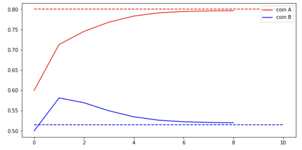
\[\hat \theta_A = 0.80\] \[\hat \theta_B = 0.45\]

Let us now imagine we don’t know the identity of the coins. We thus introduce a latent variable.

Note: for the full details, see this document.

$Z$ is the latent variable where $z_i = (z_{i1}, z_{i2}) \in \{(0,1),(1,0)\}$.

Step 1: compute likelihood

The likelihood is computed using conditional probabilities on the latent variable.

Note: the likelihood is often written $\mathbb{P}(X | \theta)$. Here we implicitly have $\mathbb{P}(X,Z) = \mathbb{P}(X,Z | \theta)$ to not overload the text with conditions.

\[\begin{align*} \text{likelihood} &= \mathbb{P}(X,Z) \\ &= \mathbb{P}(X | Z) \mathbb{P}(Z) \\ &= \prod_{i=1}^5 \mathbb{P}(\{x_i^1,...,x_i^{10}\} | z_i) \prod_{i=1}^5 \mathbb{P}(z_i) \end{align*}\]

where:

$\mathbb{P}(x_i^j | z_i) = \prod_{k=1}^2 \big( \theta_k^{x_i^j}(1-\theta_k)^{1-x_i^j} \big)^{z_{ik}}$

and:

$\mathbb{P}(z_i) = \prod_{k=1}^2 \pi_{k}^{z_{ik}}$

Finally:

\[\text{likelihood} = \prod_{i=1}^5 \prod_{j=1}^{10} \prod_{k=1}^2 \big( \theta_k^{x_i^j}(1-\theta_k)^{1-x_i^j} \big)^{z_{ik}} \prod_{i=1}^5 \prod_{k=1}^2 \pi_{k}^{z_{ik}}\] \[\text{log-likelihood} = \sum_{i=1}^5 \sum_{j=1}^{10} \sum_{k=1}^2 z_{ik} \log \theta_k^{x_i^j}(1-\theta_k)^{1-x_i^j} + \sum_{i=1}^5 \sum_{k=1}^2 z_{ik} \log \pi_k\]

Step 2: compute expectation

$\mathbb{E}[\text{log-likelihood}] = \sum_{i=1}^5 \sum_{j=1}^{10} \sum_{k=1}^2 \mathbb{E}[z_{ik}] \log \theta_k^{x_i^j}(1-\theta_k)^{1-x_i^j} + \sum_{i=1}^5 \sum_{k=1}^2 \mathbb{E}[z_{ik}] \log \pi_k$

$\mathbb{E}[z_{ik}] = … = \frac{\pi_k \sum_{j=1}^{10} \theta_k^{x_i^j}(1-\theta_k)^{1-x_i^j}}{\pi_1 \sum_{j=1}^{10} \theta_1^{x_i^j}(1-\theta_1)^{1-x_i^j} + \pi_2 \sum_{j=1}^{10} \theta_2^{x_i^j}(1-\theta_2)^{1-x_i^j}}$

Step 3: maximize expectation

$\frac{d\mathbb{E}[\text{log-likelihood}]}{d \theta_1} = 0$

=> $\sum_{i=1}^5 \sum_{j=1}^{10} \sum_{k=1}^2 \mathbb{E}[z_{ik}] (x_i^j \frac{1}{\theta_1}-(1-x_i^j) \frac{1}{1-\theta_1}) = 0$

=> $\theta_1 = \frac{\sum_{i=1}^5 \sum_{j=1}^{10} \mathbb{E}[z_{i1}] x_i^j}{\sum_{i=1}^5 10 \mathbb{E}[z_{i1}]}$ and $\theta_2 = \frac{\sum_{i=1}^5 \sum_{j=1}^{10} \mathbb{E}[z_{i2}] x_i^j}{\sum_{i=1}^5 10 \mathbb{E}[z_{i2}]}$

Numerically:

• After fixing the non latent variables $\theta_1$ and $\theta_2$, step 2 and 3 can be run iteratively.

• $\pi_1$, $\pi_2$ also need to be fixed. This doesn’t mean the latent variable is known but I believe it’s still necessary to “model” the unknown using $\pi_1 = \pi_2 = \frac{1}{2}$.

• In our example, after the first iteration:

$\mathbb{E}[z_{11}] = \frac{0.5^{10}}{0.5^{10} + 0.6^5 0.4^5} \approx 0.45$

$\mathbb{E}[z_{21}] \approx 0.80$

$\mathbb{E}[z_{21}] \approx 0.73$

$\mathbb{E}[z_{21}] \approx 0.65$

$\mathbb{E}[z_{21}] \approx 0.35$

Thus, \(\theta_1 = \frac{0.45*5+0.80*9+0.27*8+0.65*4+0.35*7}{10*(0.45+0.80+0.27+0.65+0.35)} \approx 0.71\)

• The algorithm is supposed to converge (implementation):