Mass function
The probability mass function (p.m.f.) is the histogram of the distribution, that is:
-
x-axis: values
-
y-axis: frequency
Note: the p.m.f is also called the discrete probability density function.
Density function
The probability density function (p.d.f.) is the "smoothed histogram" of the distribution.
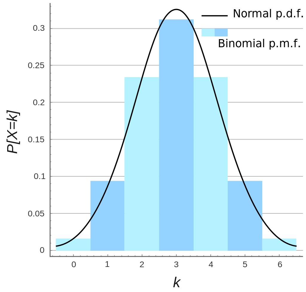
The major drawback of histograms is that they are not continuous, thus all points in the same range have the same estimated density. This can be adjusted in changing the bandwidth parameter (bins).
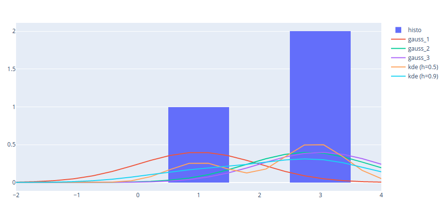
One of the common methods to solve this problem is the Kernel Density Estimation (KDE) method, also called the Parzen-Rosenblatt method. This method aims at estimating the density using the following formula:
\[\widehat f_n(x) = \frac{1}{nh} \sum_{i=1}^n K \Big( \frac{x-x_i}{h} \Big)\]$x$ is any value that we want to plot the function on.
$x_i$ are the values from the distribution to be approximated.
$h$ is the bandwidth (or smoothing parameter).
Since Kernel functions usually have inputs in $\mathbb{R}^2$, $K \Big( \frac{x-x_i}{h} \Big)$ can also be written $K(\frac{x}{h}, \frac{x_i}{h})$.
We note that the KDE estimation is an average of kernels. Thus, if the choosen kernel is continuous, the estimated density is continuous.
Using the Gaussian kernel $K(x,y) = \frac{1}{\sqrt{2\pi}\sigma} \exp \bigg( {-\frac{||x-y||_2}{2 \sigma^2}} \bigg)$, we note that the estimated density is an average of generated gaussian distributions (kernel) that are centered in $x_i$. In the graph below (extracted from KDE notebook), the distribution to be estimated is made of values $[1, 2.8, 3]$. Here the KDE method aims at building an average of three Gaussian distributions (gauss_1, gauss_2, gauss_3) centered respectively in 1, 2.8 and 3.
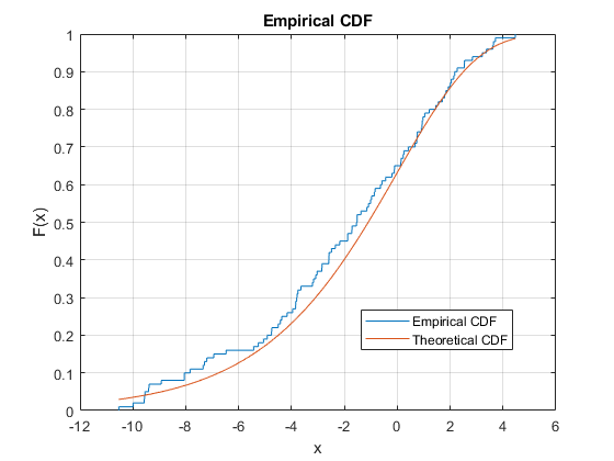
Cumulative distribution function
The cumulative distribution function (c.d.f) is given by $F_X(x)= \mathbb{P}(X < x)$.
The empirical distribution function is its estimation: $\widehat{F}_n(x) = \frac{1}{n}\{\text{number of elements} < x\}$
Quantiles and percentiles
\[\text{"quantile of } \alpha \text{"} = Q(\alpha) = \inf\{x \in \mathbb{R}: F(x) \geq \alpha \} = F^{-1}(\alpha)\] \[\text{"k-th percentile"} = Q(\frac{k}{100}) \text{ where } 0 \leq k \leq 100\]The quantile is not necessarily bounded by $0$ and $1$!

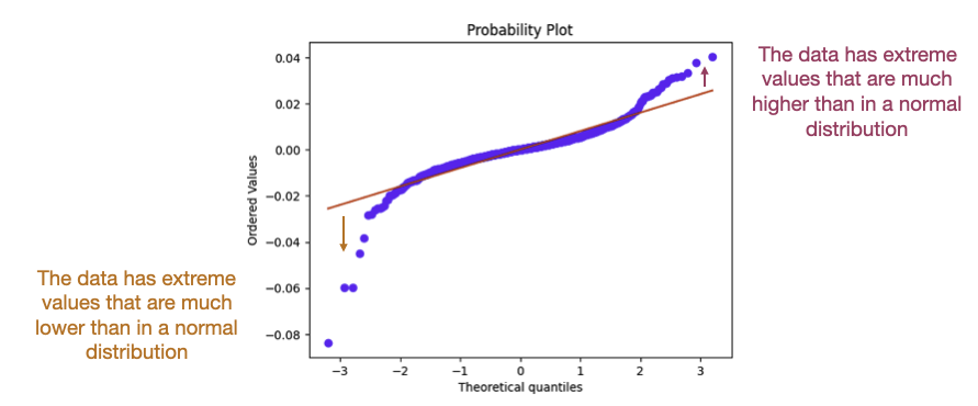
To verify the distribution of some data, the quantiles of the distribution can be compared with the ones from the theoretical distribution using the QQ plot (clear explanation by Josh Starmer). Below is the QQ plot of hourly returns of ADAUSD. We can see that the data don’t fit a normal distribution (fat tail distribution).
Normal distribution
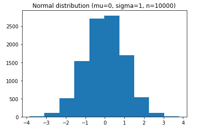
Real-life uses:
-
Human sciences (heights, Intelligence quotient,…)
-
Machine learning (kernel to give higher weights to closer neighbors)
-
Stock returns
Bernoulli distribution
\[\mathbb{P}(X=x) = \left\{ \begin{array}{ll} p & \text{if}\ x=1 \\ 1-p & \text{if}\ x=0 \end{array} \right.\]The p.m.f is expressed as
\[f(k;p) = p^k (1-p)^{1-k}\]Binomial distribution

- Repetition of Bernoulli
Real-life uses:
-
Toss a coin
-
Click or no click
Below is an example with 10000 trials, 10 tosses per trial and a probability of successes of $0.2$.
# From Bernoulli to Binomial distribution

n_bernoulli = 10 # n_size
n_binomial = 10000 # n_trials
p_bernoulli = 0.2
success_list = []

for i in range(n_binomial):
    X_bern = [bernoulli.rvs(p_bernoulli, size=1)[0] for _ in range(n_bernoulli)]
    n_fails = len(np.where(np.array(X_bern)==0)[0])
    n_successes = len(np.where(np.array(X_bern)==1)[0])
#     plt.hist(X_bern, rwidth=10, bins=3)
#     plt.xticks(range(1,2))
#     plt.show()
    success_list.append(n_successes)

plt.hist(success_list, bins=8)
plt.show()

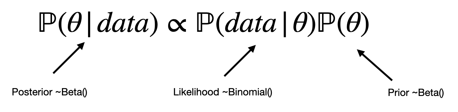
Beta distribution
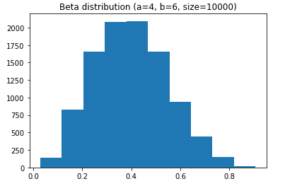
- Conjugate prior of the binomial distribution (examples at the end of this presentation):
- Represents the probability of successes, while the Binomial distribution represents the number of successes
- Seen as the continuous equivalent of the Binomial distribution
- Thanks to the above, the Beta distribution is bounded between 0 and 1
- The distribution is skewed toward the mean $\frac{a}{a+b}$
Real-life uses:
- Prior distribution in Bayesianism (successes/failures as parameters)
- Fit any distribution. Most distributions can be seen as Beta distribution with specific parameters. $\beta$ can be seen as the weight given to small values:
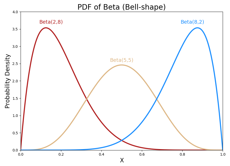
To draw a distribution knowing the mean and the standard deviation, one can use formulas to derive $\alpha$ and $\beta$.
Pareto distribution
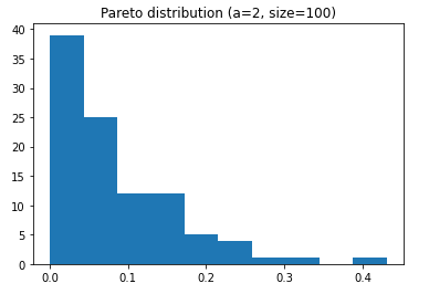
- Also known as the modelisation of the “80-20” principle: 80% of the consequences come from 20% of the causes.
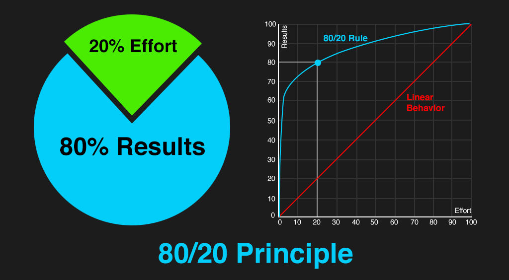
Real-life uses:
- When raising funds, often times only a few people (20%) are responsible for most of the funds (80%).
Log-normal distribution
If $X \sim \mathcal{N}(.,.)$ then $e^X \sim LN(.,.)$.
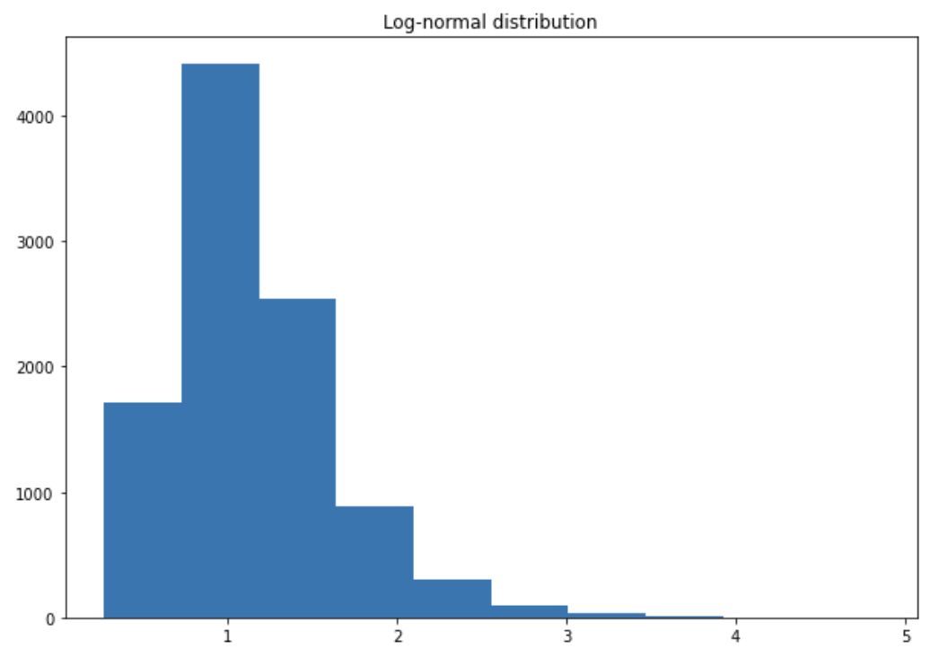
The log-normal distribution always has a positive skew (heavier right tail) i.e. larger values are distributed on a wide range. The larger the standard deviation, the heavier the tail. The mean is higher than the median because the mean is sensitive to outliers and thus pushed up by large values. The heavier the tail, the less representative is the mean.
Real-life uses:
-
In finance, returns are often assumed normally distributed and prices log-normally distributed.
-
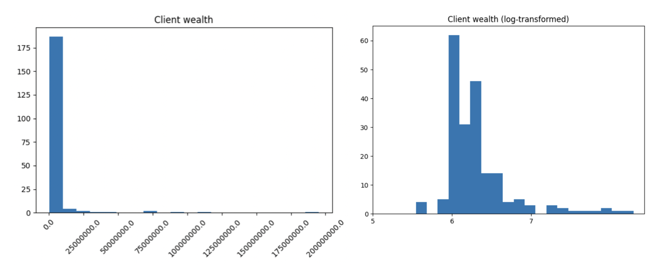
The salary distribution is heavy-tailed as showed below. Log-normal transformation is often used to improve the visual interpretation of a graph. When there are outliers with large values, the transformation shifts the low values to the right and the large observations to the left. We say the log-normal transformation “encourages the poor and penalizes the rich”. Put it differently, using a log-normal transformation reduces the impact of extreme values.
Logistic distribution
p.d.f:
\[f(x;\mu,s)=\frac{e^{-(x-\mu)/s}}{s\left(1+e^{-(x-\mu)/s}\right)^2}\]c.d.f:
\[F(x)=\frac{1}{1+e^{-(x-\mu)/s}}\]When $\mu=0$ (often the case when variables are centered),
\[F(x)=\frac{1}{1+e^{-\frac{x}{s}}} = \frac{1}{1+e^{-\gamma x}}\]where $\gamma$ is the sensitivity.
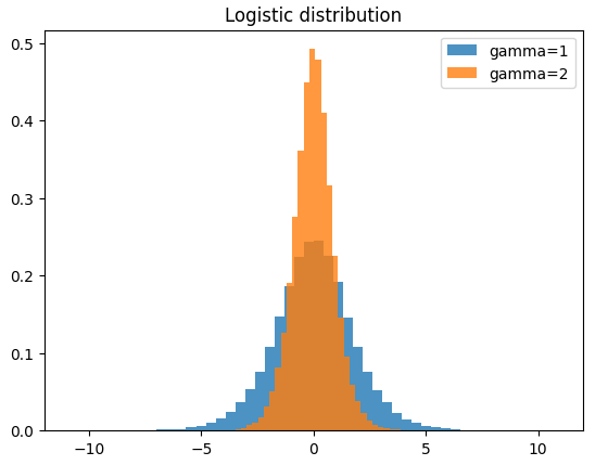
Real-life uses:
-
In NN –> logistic regression.
-
In HFT: convert trade expectation to probability of execution.
-
Anytime when we want to convert a variable to a probability.
Poisson distribution
The Poisson distribution is a discrete distribution that is often used to model an event over time.
p.m.f:
\[\mathbb{P}(X=x)=\frac{\lambda^x}{x!}e^{-\lambda}\]$\lambda$ is the expected rate of occurence of the events. In practice, it’s often estimated from past events.
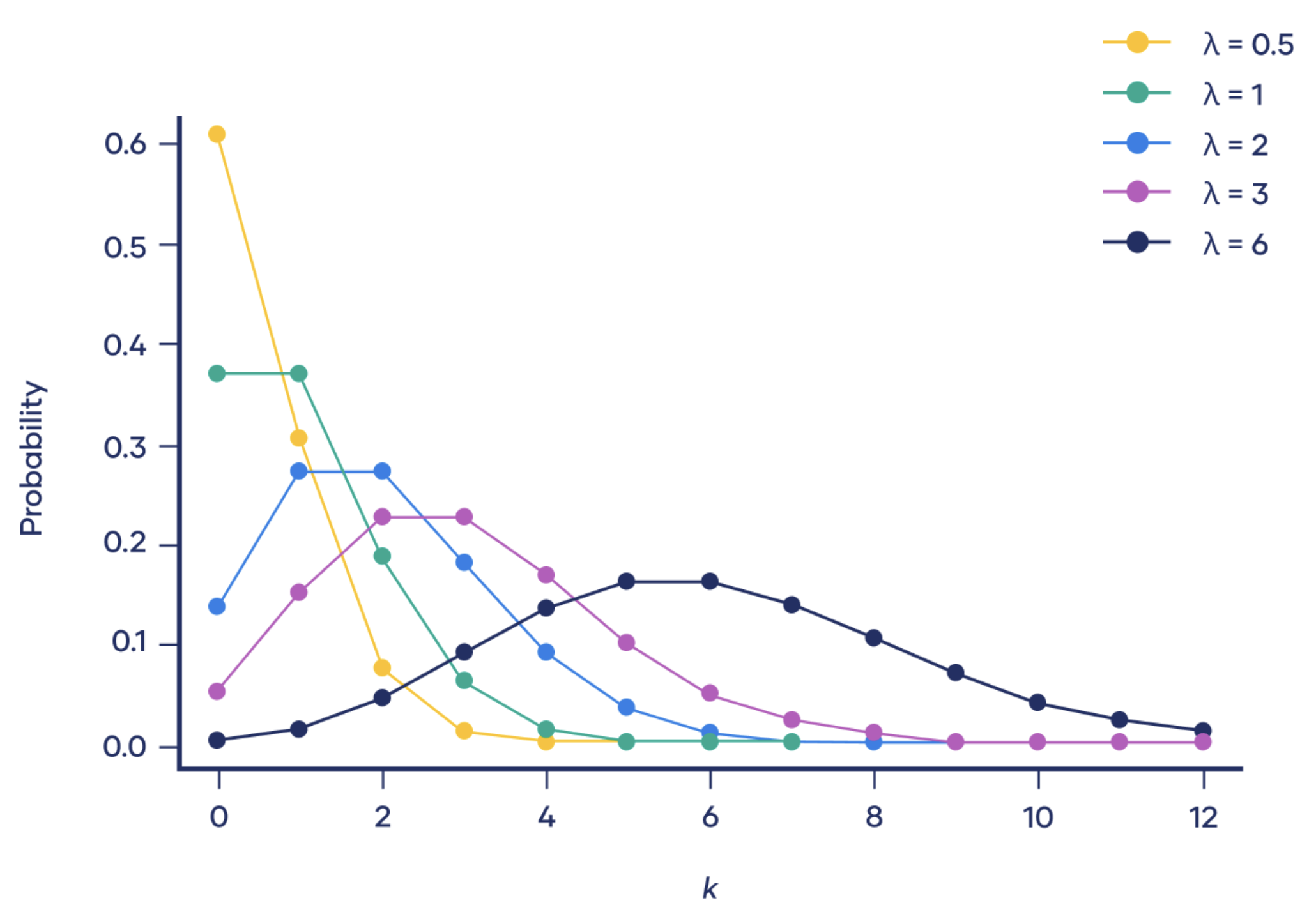
We note that the distribution looks like a normal distribution centered in lambda.
Real-life use:
-
Number of customers entering a shop.
-
Number of jumps in a financial market.
-
Number of trades that hit a specific level (HFT).