Technical analysis is the method of forecasting price movements relying on information derived from past market data (typically price, volume, low, high, etc.).

Although classical indicators like MACD, RSI, etc. are traditionally associated with either trend-following or mean-reversion behavior, any such indicator can be used for both purposes depending on the trading rules (= thresholds) applied.

E.g. RSI is traditionally used to detect mean-reversion patterns with the following rules:

RSI>70 => sell

RSI<30 => buy

But it can also be used as a trend-following indicator by inverting the rules:

RSI>70 => buy

RSI<30 => sell

There are several types of indicators:

• Trend indicators detect the market’s overall direction by smoothing -> simple MA.

• Momentum indicators measure the speed and strength of recent price movements by transforming price changes -> RSI, MACD, etc.

• Market structure indicators Market structure indicators identify key price levels and patterns where price is likely to react. -> resistances/supports, candles.

• Volatility indicators measure how widely price fluctuates -> Bollinger.

• Volume indicators measure buying and selling pressure -> OBV.

• Time-based indicators capture calendar patterns -> market opening times, current hour, etc.

Moving averages

See computation details in the associated notebook.

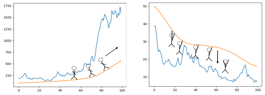
To identify a bullish/bearish trend, one can look whether the price is above/below the moving average. Using a larger window allows to detect more persistent moves.

Note: the below draw is a visual memo to remember how to detect trends with the relationship price/MA.

• prices above the MA => bullish trend

• price below the MA => bearish trend

Simple moving average

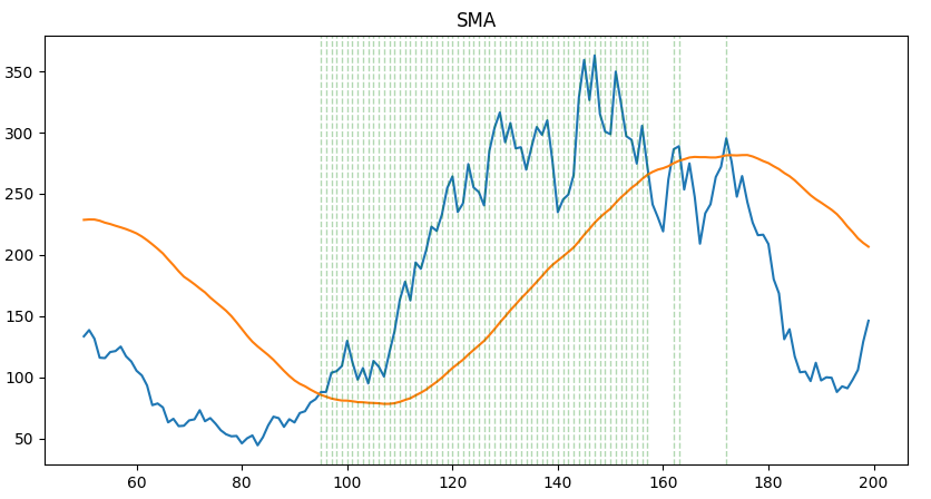
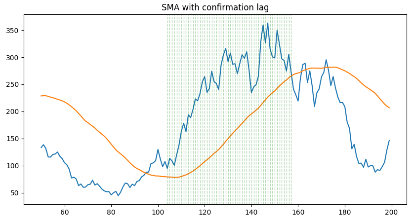
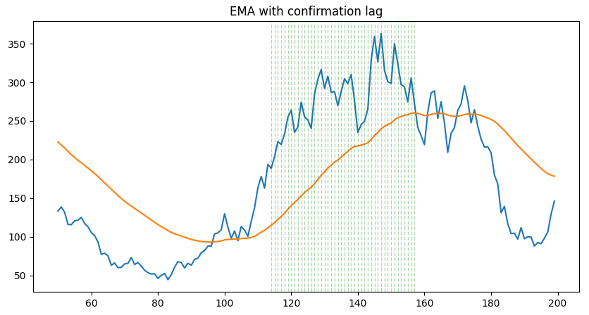
Using only a SMA is not ideal to detect persistent moves. One can use a confirmation lag to make sure the trend is here since some time.

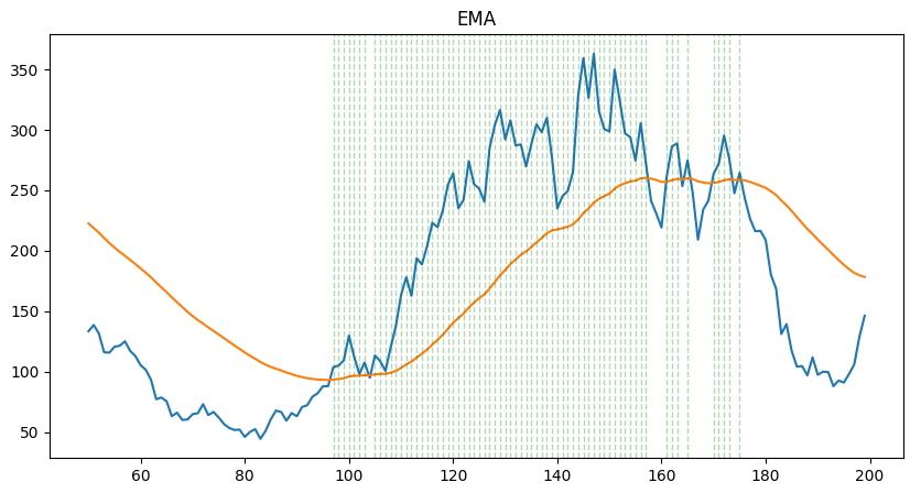
Exponential moving average

The EMA is more sensitive than the SMA (= it reverses faster). It can be compared with a SMA with a shorter window in the sense that an EMA with a long window can achieve the same sensitivity. However, the EMA is in general better because it relies on more data (bigger window).

As a reminder:

See Time Series (chapter in /Stats) to have more details.

With confirmation lag:

MA crossover

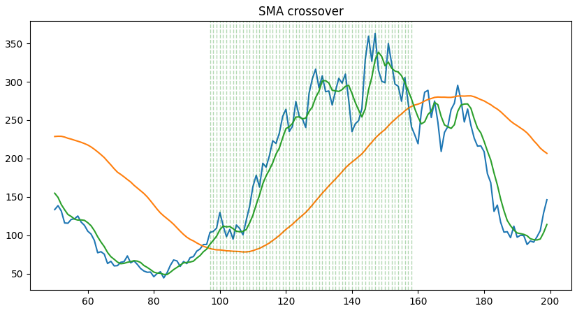
SMA crossover

Using a MA crossover can be seen as a variation of using a MA with a confirmation lag: instead of comparing all values in the lag with the long MA, we compare only one aggregated value (= average in the case of a SMA) with the long MA.

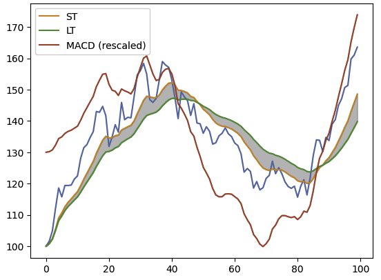
EMA crossover (= MACD)

MACD = Moving Average Convergence Divergence.

where:

• $EMA_{ST}$ is the short-term exponential moving average of the price –> moves fast

• $EMA_{LT}$ is the long-term exponential moving average of the price –> moves slow

As a reminder:

See Time Series (chapter in /Stats) to have more details.

Advantages of the MACD over a simple moving average:

• It oscillates around 0, hence it can easily be combined with other indicators to find signals.

• It shows the difference between moving averages of 2 different delays, hence, intuitively, we can better spot timing changes (e.g. a strong reversal). In other words, it responds quicker to price changes.

In the below graph, the MACD (red) is also represented by the gray areas.

The MACD crossover is a strategy that consists in using the MACD to detect buy and sell orders.

In addition to the MACD, the strategy involves another curve: the signal line.

The signal line is thus a lagged version of the MACD. When the MACD crosses the signal and end above it, it is a good indication to buy.

In the below, we use shift() to find first and lag price of a range.

lag = 3 is used to allow the crossover to happen on a range of observations to get more signals.

# MACD crossover (vectorized)

lag = 3
short_ema = df[column_price].ewm(span=12, min_periods=12).mean()
long_ema = df[column_price].ewm(span=26, min_periods=26).mean()
df['macd'] = short_ema - long_ema
df['signal_line'] = df['macd'].ewm(span=9, min_periods=9).mean()
df['signal_line_shifted'] = df['signal_line'].shift(lag)
df['macd_shifted'] = df['macd'].shift(lag)
df.loc[(df['macd']>df['signal_line']) & (df['macd_shifted']<df['signal_line_shifted']), 'is_macd_crossover_bullish_{}'.format(lag)] = True
df.loc[(df['macd']<df['signal_line']) & (df['macd_shifted']>df['signal_line_shifted']), 'is_macd_crossover_bullish_{}'.format(lag)] = True

Note: it is recommended to combine this indicator with a long term moving average (e.g. $EMA_{200}$).

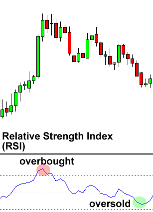
RSI

The RSI (relative strength index) is a momentum indicator that becomes high when prices have risen strongly in the last recent periods. In its traditional form, it’s used to detect mean-reverting patterns.

$RS = \text{momentum ratio} = \frac{\text{average gains}}{\text{average losses}}$

The final formula normalizes the RS to a 0-100 scale:

df['diff'] = df['prices'].diff(1)
df['up'] = 0.0
df.loc[df['diff']>0, 'up'] = df['diff']
df['down'] = 0.0
df.loc[df['diff']<0, 'down'] = df['diff'].abs()
avg_gain = df['up'].rolling(window=window).mean()
avg_loss = df['down'].rolling(window=window).mean()
rs = avg_gain/avg_loss
df['rsi'] = 100*(1-(1/(1+rs)))

The classical decision rule is:

• RSI>70 => overbought => sell

• RSI<30 => oversold => buy

Stochastic oscillator

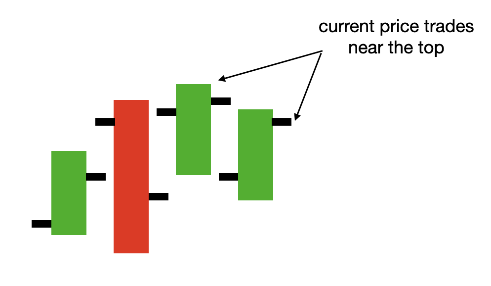
The stochastic oscillator is a momentum indicator (in its traditional form) that becomes high when the current price is near the highest level of the lookback window, which typically occurs during upward trends.. As compared with the RSI indicator, the SO indicator is more sensitive to intraperiod (e.g. 1h) extremes as it doesn’t focus on close prices only. In its traditional form, it’s used to detect mean-reverting patterns.

The denominator of $K_i\%$ should be interpreted as a scaling factor so that $0 \leq SO \leq 1$.

df['lowest_low'] = data['low'].rolling(window=window_extremum, \
	min_periods=window_extremum).min()
df['highest_high'] = data['high'].rolling(window=window_extremum, \
	min_periods=window_extremum).max()
df['stochastic_oscillator'] = \
	(df['close']-df['lowest_low'])/(df['highest_high']-df['lowest_low'])
df['stochastic_oscillator'] = df['stochastic_oscillator'].rolling(window=window_smoothing, \
	min_periods=window_smoothing).mean()