Variance

Variance theoretical formula: $\mathbb{V}[X] = \mathbb{E}[(X-\mathbb{E}[X])^2]$

Variance empirical formula: $var_n(x) = \frac{1}{n} \sum_{i=1}^n (x_i - \bar x)^2$

Variance (sample) empirical formula: $var_n(x) = \frac{1}{n-1} \sum_{i=1}^n (x_i - \bar x)^2$

The sample variance is larger than the population variance so that it takes into account of additional uncertainty .

Standard deviation

The standard deviation is the classical way to compute the volatility.

Standard deviation empirical formula: $\sigma = \sqrt{var_n(x)}$

The standard deviation is most often computed from the returns. Intuitively, it represents the “typical variation around the mean”.

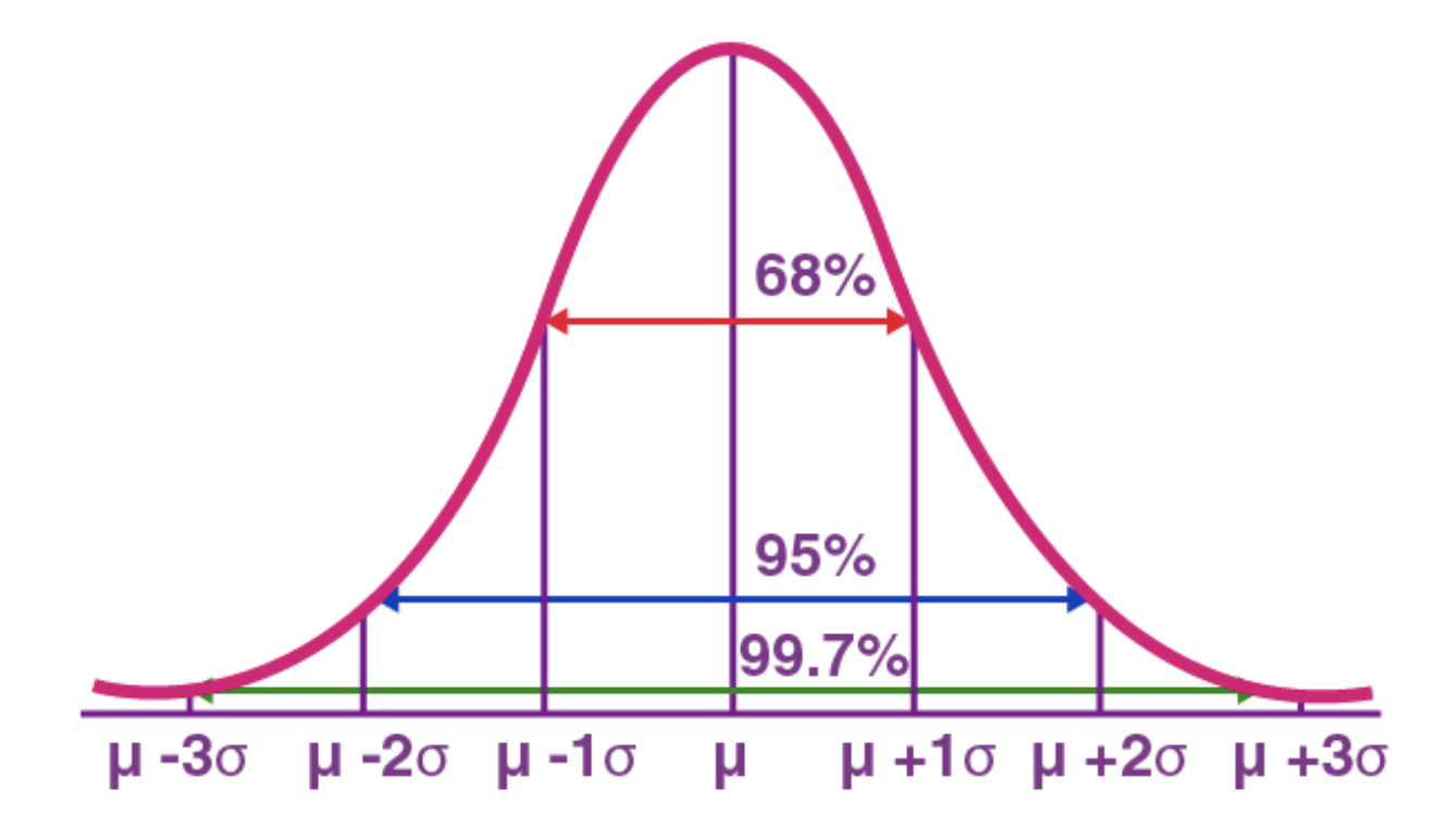
If the variable is normally distributed, the below figure is important to have an order of magnitude:

The standard deviation is important in algorithmic trading since a good trade should be profitable after fees deduction. Hence the asset move should be large enough to pay the fees.

Examples

• VIX: 15-20% (typical level in normal market environment).

Note: the VIX is a measure of the expected equity volatility.

• BTCUSD: 20% monthly (2019).

• BTCUSD: 84% annualized daily (2021).

• BTCUSD: 0.53% hourly (October 2022).

• XRPUSD: 1.17% hourly (October 2022).

VaR

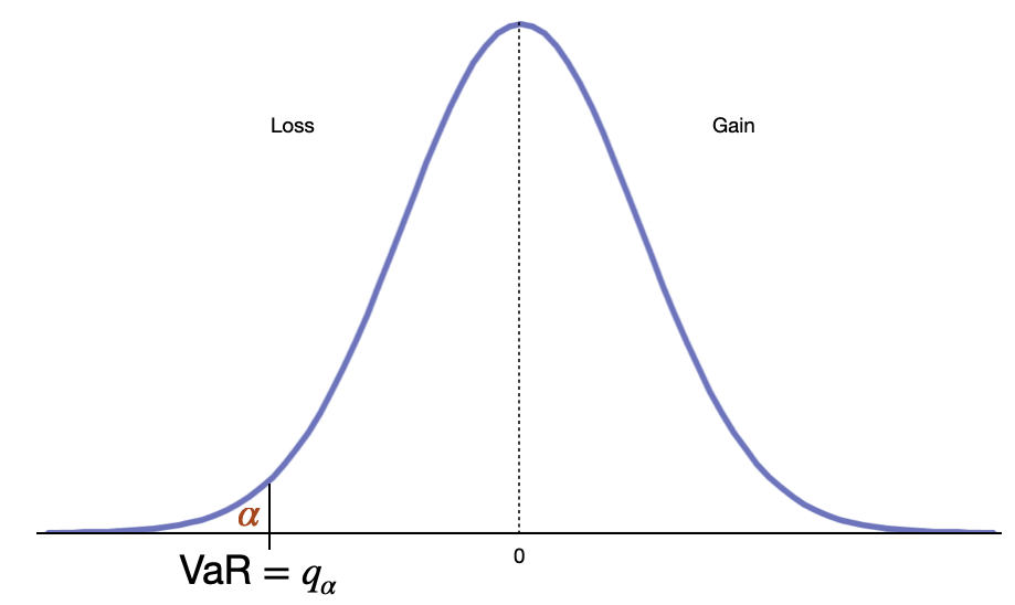
The Value-at-Risk is the maximum loss in extreme scenarios.

Most often, it represents the loss amount that one would face with a certain probability $\alpha$ over a certain length of time. Hence, it combines 3 aspects: amount, probability, time window.

Mathematically:

\[VaR_\alpha(X) = \inf \{ x \in \mathbb{R}, F_X(x) > \alpha \}\]

where $X$ are the returns of the strategy over a certain time window, and $F_X$ its cumulative distribution function.

From a statistical perspective, the VaR is simply the quantile associated with a certain $\alpha$. As a reminder, the quantile function is the inverse of the cumulative density function.

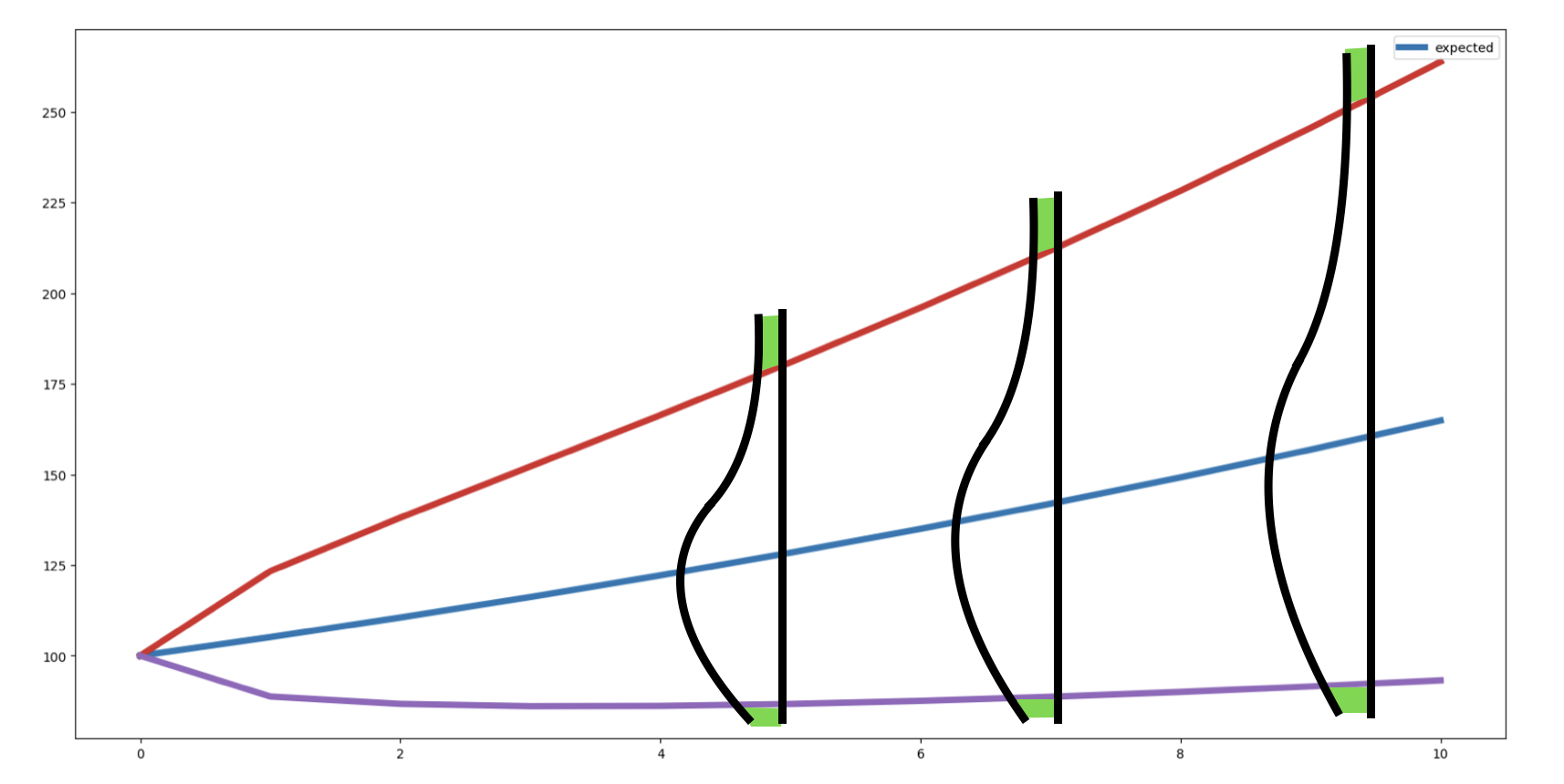
To compute the VaR in the case of a GBM, see the Wealth planning section where we compute the quantiles at each step of the projection.

MAR

The mean of absolute returns (MAR) can be more relevant in some cases as it reflects the typical variation. The standard deviation is often used as it penalizes more the big moves. E.g. a stock that does [-1%,1%,-10%,1%] would have MAR=3.3% and STD=4.6%. Also, the STD is about the deviation around the mean: [-1%,-1%,-1%,-1%] would give MAR=1% but STD=0% (the stock does not move around the mean). Moreover, the standard deviation has nice statistical properties e.g. it is used in the central limit theorem.

ATR

The Average True Range (ATR) is often more informative for trading rules since it accounts not only for close-to-close returns (like the standard deviation) but also intraperiod highs, lows, and gaps — giving a fuller picture of realized market movement. For example, if an asset shows returns of [+1%, +1%, +1%, +1%], it may appear non-volatile, yet this ignores the price fluctuations that may have occurred within each period.

\[TR = \max(\text{High}-\text{Low}, | \text{High} - \text{Previous close} |, | \text{Low} - \text{Previous close} |)\] \[ATR = \frac{\sum TR_{14}}{14}\]