Moment 1 = mean

Moment 2 = variance

\[\mu_2 = \mathbb{V}[X] = \mathbb{E}[(X-\mathbb{E}[X])^2]\] \[\hat \mu_2 = \sigma^2 = \frac{1}{n} \sum_{i=1}^{n} (x_i-\bar x)^2\]

Moment 3

\[\mu_3 = \mathbb{E}[(X-\mathbb{E}[X])^3]\] \[\hat \mu_3 = \frac{1}{n} \sum_{i=1}^{n} (x_i-\bar x)^3\] \[\text{skewness} = \text{normalized 3rd moment} = \frac{\mu_3}{\sigma^3}\]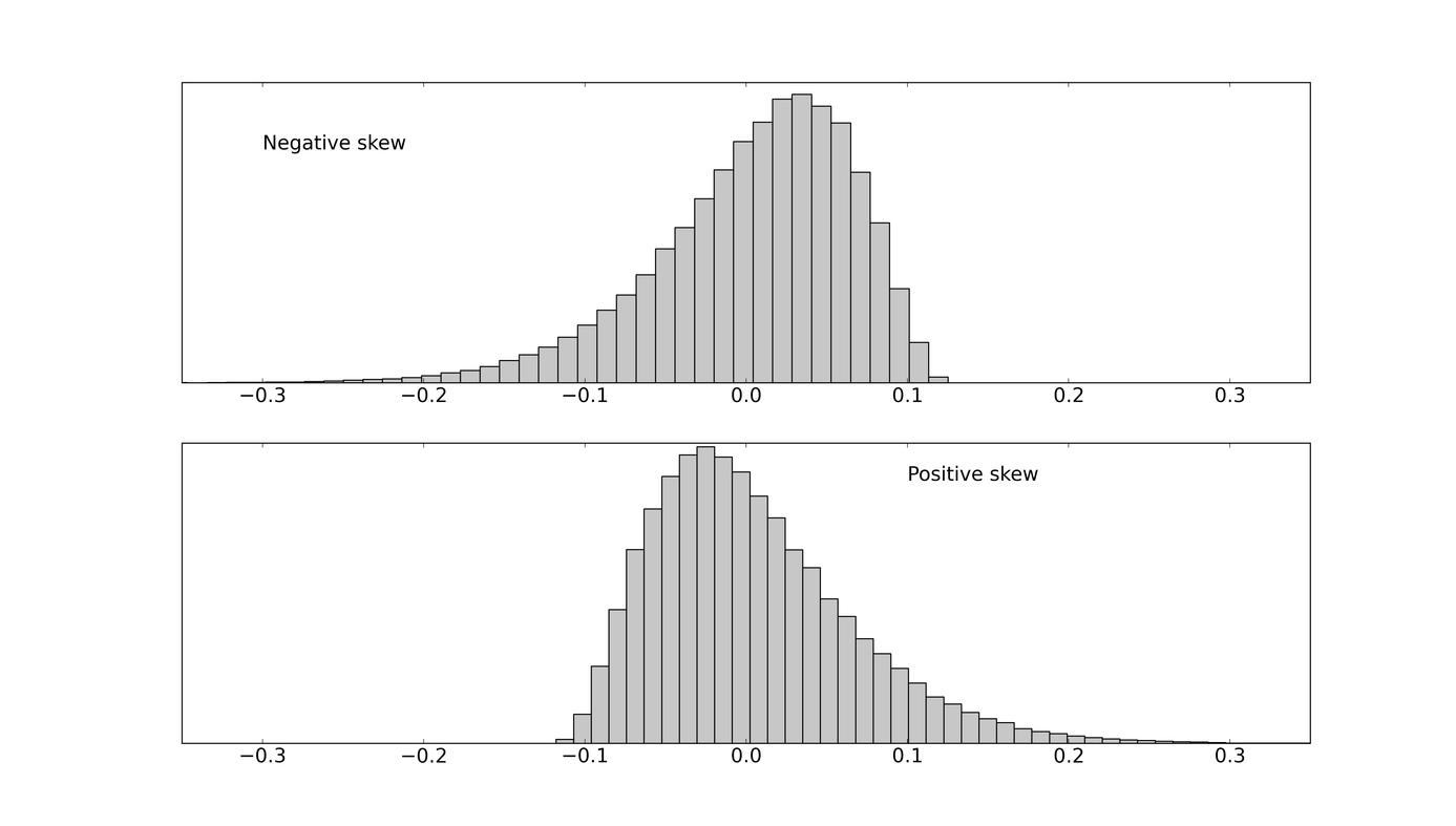

Negative skewness = fatter left tail. More unusual events when the market is bearish.

Positive skewness = fatter right tail. More unusual events when the market is bullish. Memo: “positive” skewness -> generally favorable for investors because it implies more frequent extreme positive moves (not true if the investor enters short positions).

Moment 4

\[\mu_4 = \mathbb{E}[(X-\mathbb{E}[X])^4]\] \[\hat \mu_4 = \frac{1}{n} \sum_{i=1}^{n} (x_i-\bar x)^4\] \[\text{kurtosis} = \text{normalized 4th moment} = \frac{\mu_4}{\sigma^4}\]

High kurtosis = fat tails. More unusual events.

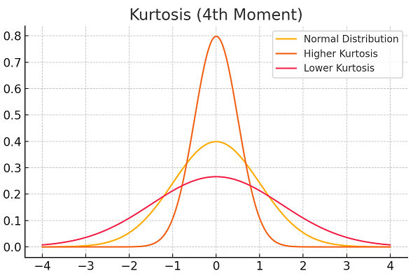
Note: the normal distribution has kurtosis equal to 3. Hence many packages return $\text{excess kurtosis} = \text{kurtosis}-3$.

Example

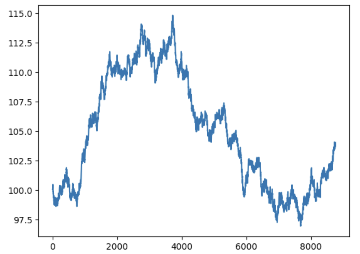
Prices generated with a pure random normal distribution (skew=0.01, kurtosis=0.04):

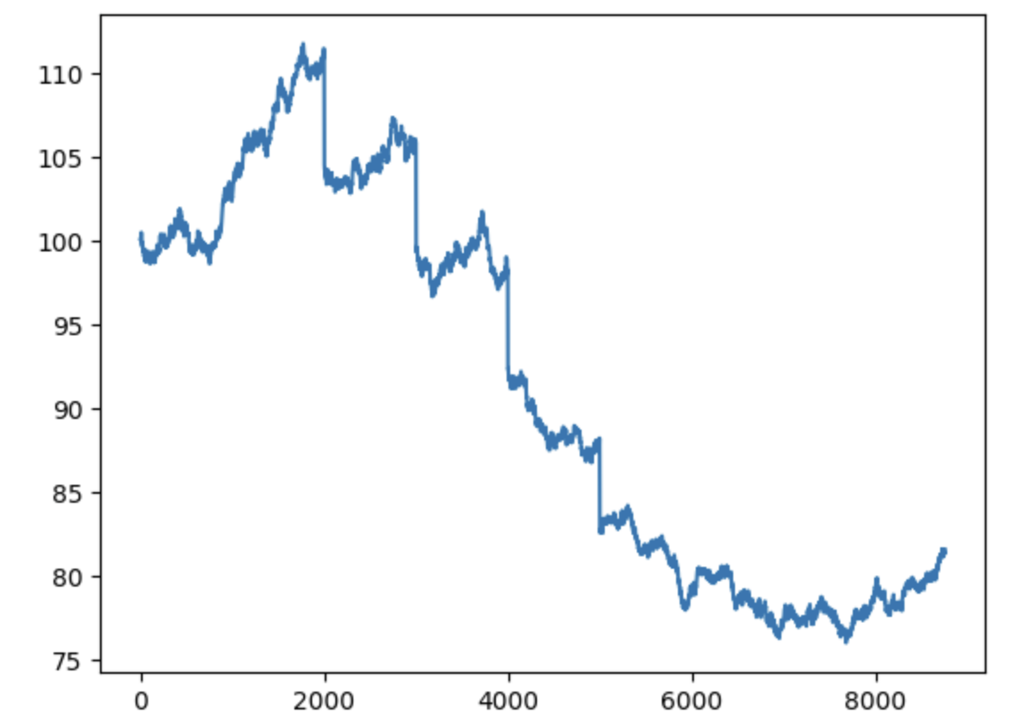
After adding strong negative jumps (skew=-20.91, kurtosis=747.14):

General remarks

Fat tails generally make modeling harder because:

• historical relationships break more often,

• rare events have little training data,

• estimation becomes unstable.

However, fat-tailed regimes can also create:

• strong inefficiencies,

• momentum bursts,

• volatility dislocations,

• panic/recovery dynamics,

• behavioral overreactions.

A practical approach is therefore not to completely avoid fat-tailed regimes, but to adapt the strategy to them. In “normal” regimes, the model can focus on stable statistical relationships and tighter risk controls. In fat-tailed regimes, it is often better to switch to more robust behavior: reduce leverage, widen risk thresholds, rely on simpler/high-conviction signals,