Multiplicative VS additive

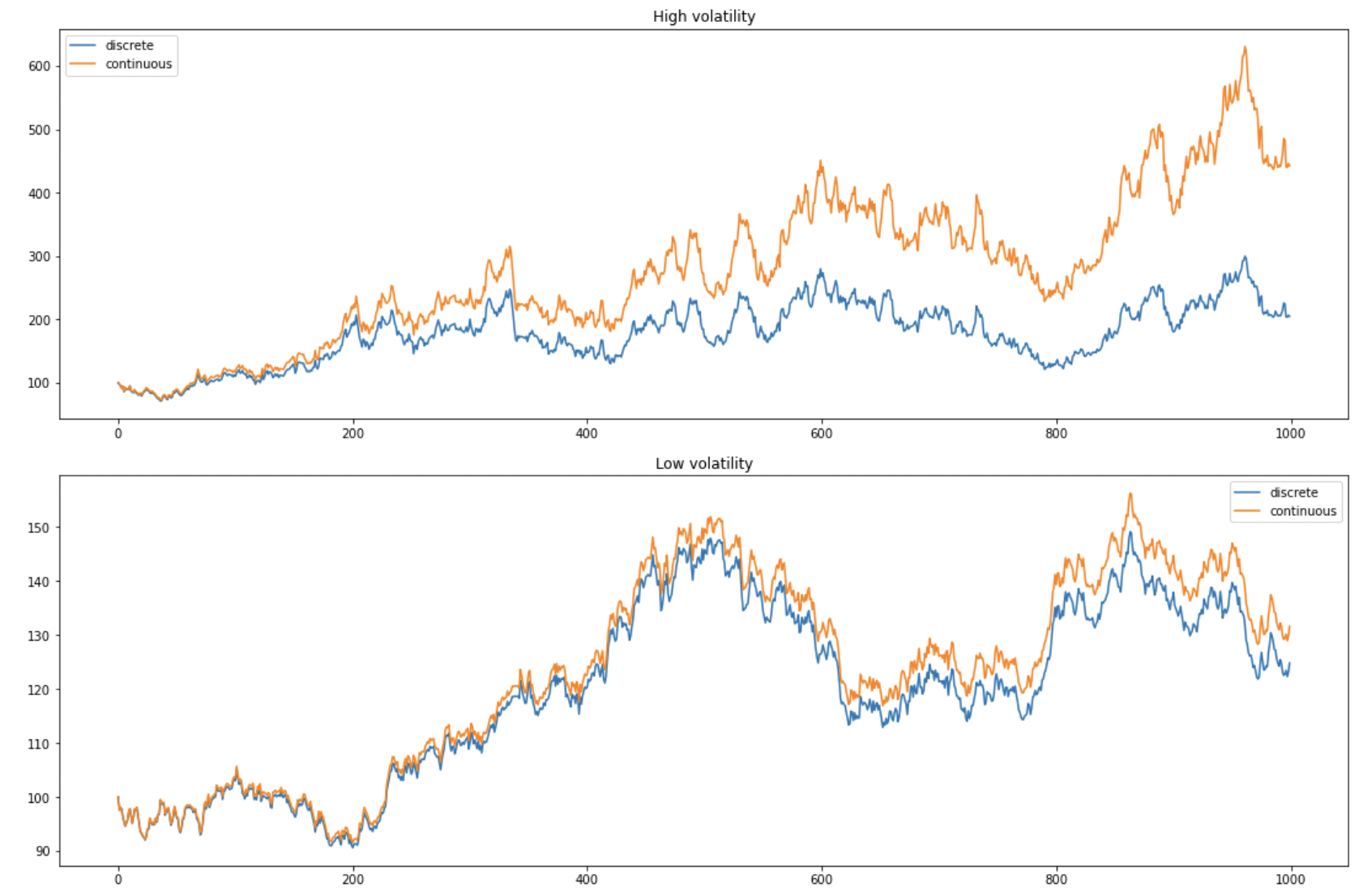
Discrete returns are multiplicative while continuous returns are additive. For this reason, we tend to prefer to use continuous returns when there is a small volatility w.r.t. the considered period. Indeed, it becomes simpler for mental calculations:

High volatility
$P_0 = 100$
$P_1 = 120$ => $R_1 = +20\%$
$P_2 = 60$ => $R_2 = -50\%$
Total variation = $\frac{P_2}{P_0}-1 = -40\% \neq R_1 + R_2$
Low volatility
$P_0 = 100$
$P_1 = 101$ => $R_1 = +1\%$
$P_2 = 99$ => $R_2 = -1.9\%$
Total variation = $\frac{P_2}{P_0}-1 = -1\% \approx R_1 + R_2$

np.random.seed(1)
n = 1000
returns = np.random.normal(0,.04,n)
returns[0] = 0

cumul_returns_discrete = (1+returns).cumprod()-1
prices_discrete = 100*(1+cumul_returns_discrete)

cumul_returns_continuous = np.cumsum(returns)
prices_continuous = 100*np.exp(cumul_returns_continuous)

x = np.arange(n)
fig, (ax1, ax2) = plt.subplots(2,figsize=(15,10), constrained_layout = True)
ax1.plot(x, prices_discrete, label='discrete')
ax1.plot(x, prices_continuous, label='continuous')
ax1.set_title('High volatility')
ax1.legend()

returns = np.random.normal(0,.01,n)
returns[0] = 0

cumul_returns_discrete = (1+returns).cumprod()-1
prices_discrete = 100*(1+cumul_returns_discrete)

cumul_returns_continuous = np.cumsum(returns)
prices_continuous = 100*np.exp(cumul_returns_continuous)

ax2.plot(x, prices_discrete, label='discrete')
ax2.plot(x, prices_continuous, label='continuous')
ax2.set_title('Low volatility')
ax2.legend()

plt.show()

Real life

Even though most financial models assume continuity, the “true” nature of prices is discrete.

E.g. stock prices change only when there are trades, which happen at fixed points of time.

E.g. car prices will never be 10000.020384, rather 10000.

Relationship

$R$ being the discrete return, $r$ the continuous return, we have (trivial proof):

Discrete returns can be converted to continuous before using a model that is based on continuous returns. That way we make sure the results are true in the discrete and continuous cases.

E.g. a portfolio has an expected discrete return of $R = 3\%$. We want to forecast its return in the next years using a Geometric Brownian Motion (GBM). Since GBM is a continuous model, we first convert the return to continuous $r = \ln(1+3\%) = 2.96\%$. $r$ is thus used in the GBM but $R$ can also be used to check the result at maturity: after $T$ years, the portfolio’s expected return will be $S_0(1+R)^{T}$. This matches the continuous formula $S_0e^{rT}$.