Termsheet (core components)

10NC1 USD Callable Fixed-Rate Note, 6.90% p.a.

Investor exposure

• Long a 10Y 6.90% bond of the issuer -> vanilla
• Short a Bermudan call on that bond -> exotic

In practice, the bond part is decomposed into two components:

• Long a zero-coupon bond of the issuer (the 100 at maturity) -> vanilla
• Long a strip of annual 6.90% coupons -> vanilla

Calibration step

The Hull-White model, $dr_t = (\theta(t) - a\, r_t)\,dt + \sigma\, dW_t$, fits today’s yield curve exactly. Only two parameters, $a$ (mean reversion) and $\sigma$ (volatility of the short rate) are calibrated to option prices. The volatility is deterministic in this model.

The Hull-White dynamics describe how the short rate, and therefore the whole yield curve, can evolve up to any future date e: this is what we need to value the issuer’s decision at each call date.

All steps

1. Termsheet: define a 10NC1 USD callable note: annual fixed coupon, issuer can repay at par every year from year 1 to year 9.
2. Market data: download the Treasury curve and the single-A credit spread (FRED), plus IEF/TLT option chains and the MOVE index (Yahoo).
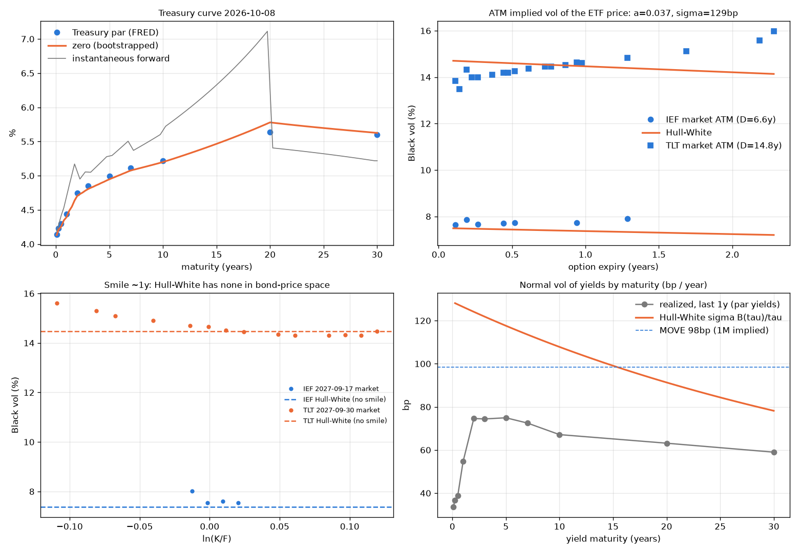
3. Zero curve: bootstrap the Treasury par yields into discount factors, which fixes $\theta(t)$ so the model reprices today’s curve exactly.
4. ETF mapping: treat each bond fund as a zero-coupon bond whose maturity is estimated by regressing its returns on yield changes.
5. Implied vols: get forwards from put-call parity, invert Black-76 on out-of-the-money quotes, and take the at-the-money vol for each expiry.
6. Calibration: fit a and $\sigma$ to those vols with the closed-form Hull-White bond option formula.
7. Pricing: build the trinomial tree and roll back with V = min(continuation, 100) + coupon at each call date, then solve the fair coupon.
8. Sanity checks: confirm the tree reprices the curve, matches the closed form (Jamshidian) for European calls, recovers the zero-vol limit, and converges as the time step shrinks.
9. Sensitivities: bump and reprice to get duration, convexity, key-rate DV01, vega, CS01 and mean-reversion risk, which shows the note’s negative convexity.

Finite differences

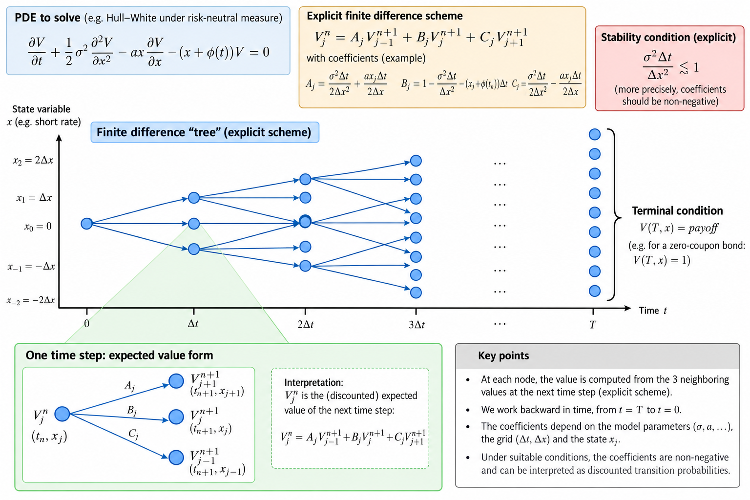
The finite difference method solves the Hull-White PDE numerically: it replaces the derivatives by differences on a grid (time x short-rate points) and goes backward from maturity. It suits models with few state variables (here one: the short rate). The explicit scheme computes each node from its 3 neighbours at the next date (up, middle, down), like a trinomial tree, but is only stable for small time steps; implicit schemes are stable for any time step.

The explicit finite difference scheme works like the trees commonly used in pricing, such as binomial trees for American options: values are computed backward from maturity, and the discounted expected value is calculated at each node.