Walk forward optimization is the cross validation method that is commonly used to calibrate time series.
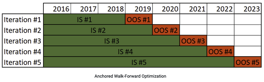
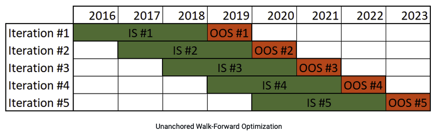
In this configuration, the out-of-sample data should NOT be used to select the right parameters / strategy. It should be run once only at the end and the results should not be used to tune further the strategy. Tip: the out-of-sample run should be used as a “blind” test i.e. we pretend we have not seen it so it’s like no decision can be taken based on its results. The only decision that can be made after seeing the out-of-sample results is to change completely the strategy or not.
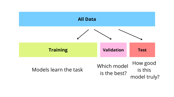
A validation set can be used to compare rivalling approaches.
E.g. in a multi time series indicators strategy:
- Train set: we find the best indicators’ parameters (e.g. rolling window).
- Validation set: we keep the parameters that gives the best results.
- Test set: final confirmation to make sure the parameters work well.
# anchored walk-forward optimization
from sklearn.model_selection import TimeSeriesSplit
tscv = TimeSeriesSplit(n_splits=3, test_size=int(0.2*X.shape[0]))
dict_thresholds = {}
for threshold in np.linspace(0.05,.5,10):
    bad_threshold = False
    precision_list = []
    f1_list = []
    for i, (train_index, test_index) in enumerate(tscv.split(X)):
        X_train = X.iloc[train_index]
        y_train = y.iloc[train_index]
        X_test = X.iloc[test_index]
        y_test = y.iloc[test_index]
        clf.fit(X_train, y_train)
        prob_pos = clf.predict_proba(X_test)[:,1]
        # we don't consider the threshold if it gives less than 5 trades
        if np.sum(np.where(prob_pos>=threshold, 1, 0))<5:
            bad_threshold = True
            break
        precision = metrics.precision_score(y_test, np.where(prob_pos>=threshold, 1, 0))
        f1 = metrics.f1_score(y_test, np.where(prob_pos>=threshold, 1, 0))
        precision_list.append(precision)
        f1_list.append(f1)
    if not bad_threshold:
        # average to have an aggregate score across the folds
        dict_thresholds[threshold] = (np.mean(precision_list), np.mean(f1_list))
Sharpe ratio
The Sharpe ratio is the most common way to assess the profitability of a strategy.
\[\text{Sharpe} = \frac{\mu_{portfolio}-\mu_{risk-free}}{\sigma_{portfolio}}\]Note (1): make sure that $\mu$ and $\sigma$ are on the same scale!
Note (2): as stated in Hull, it is common to use the Treasury bills as risk-free rate. However, this rate is artificially low because financial institutions must purchase them for a regulatory requirements (so prices increase and yields decrease). In practice, derivatives traders use the LIBOR rate.
Note (3): when comparing strategies, it is common to not adjust with the risk-free return (source RL).
When $\text{Sharpe} = 1.0$, the risk is perfectly rewarded by the performance.
A good annualized Sharpe ratio would start from 0.8.
ret_free = .05 # annualized
ret_free_daily = ret_free/252

ret_daily = pd.DataFrame(portfolio_values).pct_change(periods=1).mean().values[0]
vol_daily = pd.DataFrame(portfolio_values).pct_change(periods=1).std().values[0]

sharpe = np.sqrt(252)*(ret_daily-ret_free_daily)/vol_daily
Example
Interesting chart of the BTC rolling 52 week Sharpe ratio:
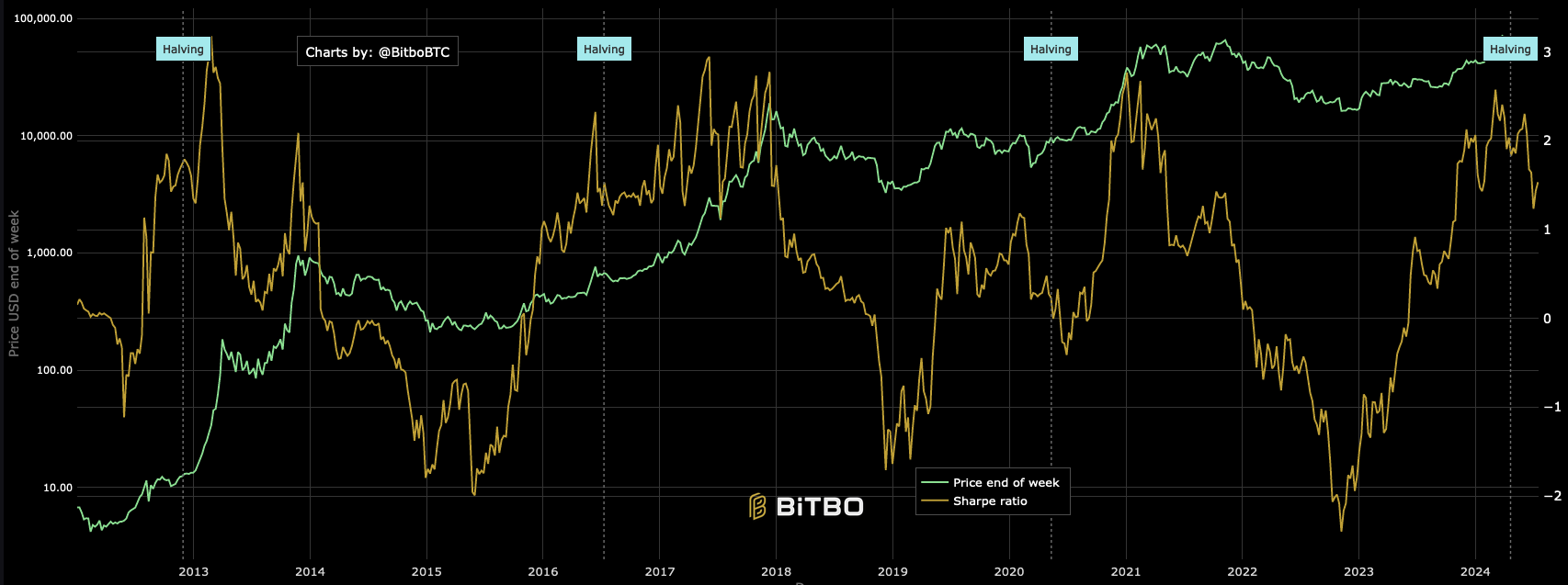
As we can see, the SR can go as high as ~3.0. However, the metric itself is quite volatile and can also be highly negative. Source: bitbo.io.
Limits
One of the main limits of the SR is that it penalizes high volatile periods no matter if the direction is profitable or not. A common alternative is the Sortino ratio.
One of the main limits of the SR is that it penalizes high volatile periods no matter if the direction is profitable or not. A common alternative is the Sortino ratio.
Cumulative return
TODO
Limits
The cumulative return can be prone to overfitting (see limits of expected gain below).
Average return
TODO
Hit ratio
The hit ratio is the percentage of successful trades on a given timeframe.
Note: to be fully accurate, the hit ratio should be computed taking the fees into account.
Limits
The hit ratio doesn’t take the magnitude of the gains/losses into account. In other words, a strategy with a high hit ratio can be very bad if it wins small and losses big. Conversely, a strategy can actually be profitable if it often loses small but wins big. One can mitigate this issue computing the hit ratio using take-profit and stop-loss levels.
Using the expectancy (see below), the break-even hit ratio should balance out: \(\text{break-even hit ratio}*(\text{take profit}-\text{fees})-(1-\text{break-even hit ratio})*(\text{stop loss}+\text{fees}) = 0\)
This leads to the following formula to compute the break-even hit ratio:
\[\text{break-even hit ratio} = \frac{\text{stop loss}+\text{fees}}{\text{take profit}+\text{stop loss}} = \frac{SL+F}{TP+SL}\]E.g. for TP=1%, SL=0.5% and F=0.3%, the required hit ratio so that the strategy gets profitable is 53.33%.
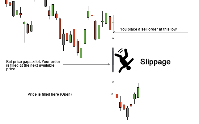
Note: this break-even hit ratio doesn’t take slippage into account. Slippage happens when the executed price is very different from the expected price. It can impact the profitability in real life. Indeed, the above computation assumes that a failed trade will be closed exactly at -2%. However, in reality we may not be able to execute the trade before it reaches -3%.
The slippage can impact the P&L negatively and positively (although less frequent). It can be eliminated using only limit orders (instead of market orders), however it introduces a risk of not getting filled.
Expected gain
The expected gain is the average gain made on each trade. It has the advantage of combining the hit ratio and the magnitude of the gains/losses.
\[\mathbb{E}[G] = \text{average gain}*\text{hit ratio}+\text{average loss}*(1-\text{hit ratio})\]Note: to be fully accurate, average gain, average loss and hit ratio should be computed taking the fees into account.
Limits
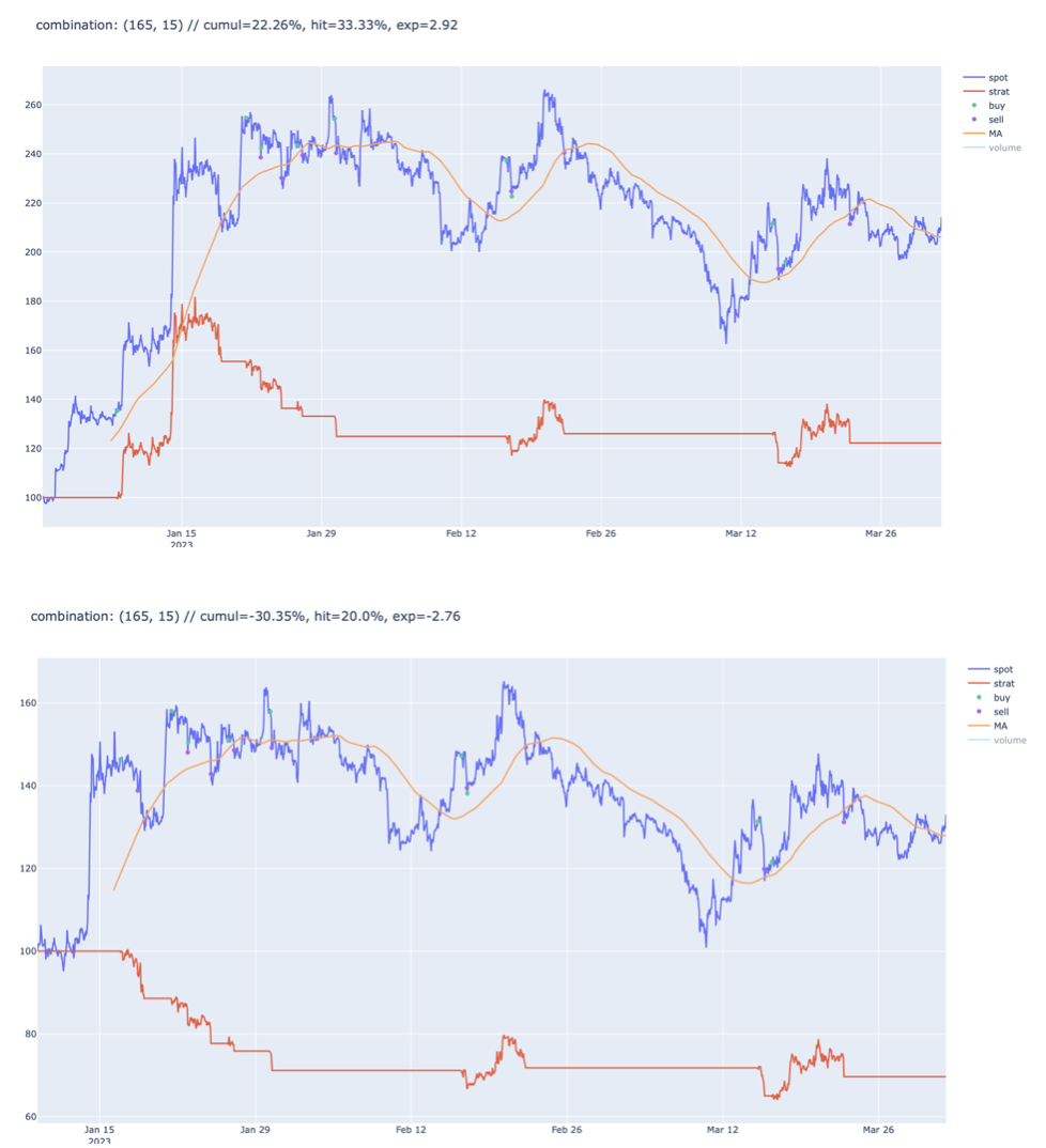
The expected gain can be prone to overfitting. In the below figures, we tested a simple moving average strategy on 2 timeframes where the second timeframe is equal to the first timeframe with a small delay. The expected gain is positive in the first scenario and negative in the second. We can also see that the hit ratio is lower than 50% in both scenarios, which should encourage us to consider both metrics when assessing the strategy.
Expected return
The expected return is also used to assess the profitability of a strategy. Example:
A hourly strategy consists in trading an asset that has a hourly volatility of 1.22%.
The strategy has a success rate of 55%.
Say the strategy runs without interruption for one month. It means that, in one month, \(30*24*0.55=396\) trades are correct and \(30*24*0.45=324\) are wrong.
$\mathbb{E}[R] = (1+1.22\%)^{396}(1-1.22\%)^{324}-1=128\%$ !
This looks very impressive, however assuming 0.2% fees paid at each trade:
$\mathbb{E}[R] = (1+1.22\%-0.2\%)^{396}(1-(1.22\%+0.2\%))^{324}-1=-46\%$
In order to achieve a minimum return, one could solve the following equation to find the required success rate:
$\mathbb{E}[R] = (1+1.22\%-0.2\%)^{720x}(1-(1.22\%+0.2\%))^{720-720x}-1>2\%$ => $x = 63\%$.