SVM

Margin

This idea of SVM is to separate data as best as possible using a margin.

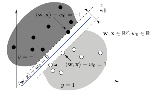
Three planes:

- $H_1: \omega^Tx+b=1$

- $H: \omega^Tx+b=0$

- $H_{-1}: \omega^Tx+b=-1$

Computing $H_1 - H_{-1}$ we get:

$(x_1-x_{-1})\omega^T=2$

=> $||x_1-x_{-1}||=\frac{2}{||\omega||}$

The SVM problem starts with a margin maximization. We want to maximize the distance between $x_1$ and $x_{-1}$ and it is equivalent to minimizing $||\omega ||$. Thus the optimization problem is written as such:

$min_{\omega,b}~\frac{1}{2}\|\omega\|^2$

$s.t.~y_i(\omega^Tx_i+b) \geq 1$ $i=1,...,n$

Primal formulation

The above problem reflects the case when all data are perfectly separable, this is not true in practice. We thus add an error term $\xi_i$ for each observation. This leads to the primal formulation of the problem:

$min_{\omega,b, \xi}~\frac{1}{2}\|\omega\|^2+C\Sigma_{i=1}^{n}\xi_i$

$s.t.~y_i(\omega^Tx_i+b) \geq 1 - \xi_i$ $i=1,...,n$

$\xi_i \geq 0$ $i=1,...,n$

Note: the problem can be rewritten with the hinge loss function

$y_i(\omega^Tx_i+b) \geq 1 - \xi_i => \xi_i \geq 1 - y_i(\omega^Tx_i+b)$

$~~~~~~~~~~~~~~~~~~~~~~~~~~~~ => \xi_i \geq 1 - y_i(\omega^Tx_i+b) \geq 0$ since $\xi_i \geq 0$

$~~~~~~~~~~~~~~~~~~~~~~~~~~~~ => \xi_i = max(0, 1 - y_i(\omega^Tx_i+b))$

$~~~~~~~~~~~~~~~~~~~~~~~~~~~~ => \xi_i = (0, 1 - y_i(\omega^Tx_i+b))_+$

$=> \xi_i = hinge(f(x))$ where $hinge$ is the Hinge loss function

$hinge(f(x)) = (1 - yf(x))_+$

Lagrange

We can write this problem using Lagrange formulation, that is, integrating the constraints into the main formula:

$\mathcal{L}(\omega,b,\xi, \alpha, \mu) = \frac{1}{2}\omega^T\omega+C\Sigma \xi_i + \Sigma \alpha_i (1-\xi_i - y_i(\omega^Tx_i+b)) - \Sigma \mu_i \xi_i$

$\alpha_i, \mu_i \geq 0$

First order conditions:

$\frac{\partial\mathcal{L}}{\partial\omega} = 0 => \omega - \Sigma \alpha_i y_i x_i = 0 => \omega = \Sigma \alpha_i y_i x_i$

$\frac{\partial\mathcal{L}}{\partial b} = 0 => -\Sigma \alpha_i y_i = 0$

$\frac{\partial\mathcal{L}}{\partial \xi_i} = 0 => C - \alpha_i - \mu_i = 0 => \alpha_i = C - \mu_i$

Since $\alpha_i, \mu_i \geq 0$ we have $C \geq \alpha_i \geq 0$

Dual formulation

We can rewrite the problem using the first order conditions above:

$\mathcal{L}(\omega,b,\xi, \alpha, \mu) = \frac{1}{2}(\Sigma \alpha_i y_i x_i)^T(\Sigma \alpha_i y_i x_i)+C\Sigma \xi_i + \Sigma \alpha_i - \Sigma \alpha_i \xi_i - \Sigma \alpha_i y_i (\Sigma \alpha_i y_i x_i)^T x_i - \Sigma \alpha_i y_i b - \Sigma \mu_i \xi_i$

$~~~~~~~~~~~~~~~~~~ = -\frac{1}{2}(\Sigma \alpha_i y_i x_i)^T(\Sigma \alpha_i y_i x_i) + \Sigma(C - \alpha_i - \mu_i)\xi_i + \Sigma \alpha_i - \Sigma \alpha_i y_i b$

$~~~~~~~~~~~~~~~~~~ = -\frac{1}{2}\Sigma_{i,j} \alpha_i \alpha_j y_i y_j x_i^T x_j + \Sigma \alpha_i$

The problem is convex with lineary inequality constraints, we can apply the saddle point theorem.

Note: a point is saddle if it’s a maximum w.r.t. one axis and a minimium w.r.t. another axis

The saddle theorem allows us to solve the problem $min_\omega max_\alpha$ as $max_\alpha min_\omega$

This leads to the problem in its dual formulation:

$max_\alpha~~-\frac{1}{2}\Sigma_{i,j} \alpha_i \alpha_j y_i y_j x_i^T x_j + \Sigma \alpha_i$

$s.t.~~0 \leq \alpha_i \leq C~~i=1,...,n$

Using the above expression of $\omega$ (optimal condition), the classification function is:

$f(x)=sign(\Sigma \alpha_i y_i x_i^T x + b)$

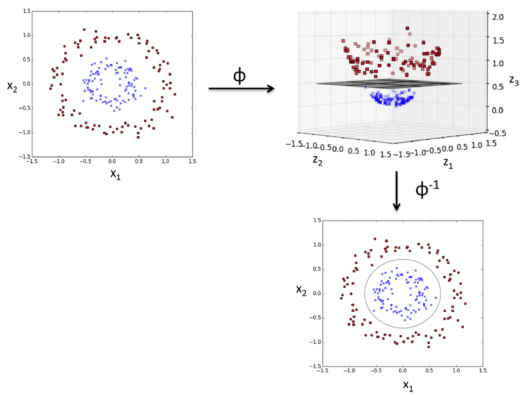
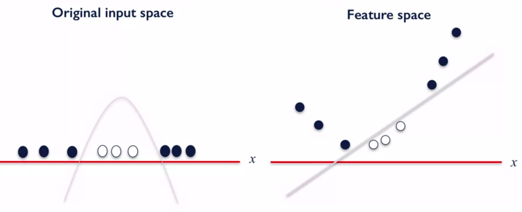
Kernel

Kernels are used when separation is non linear.

Recall the primal formulation:

When separation is non linear, we set $\phi$ as a non linear transformation. The constraint becomes:

$y_i(\omega^T\phi(x_i)+b) \geq 1 - \xi_i~~i=1,…,n$

Dual formulation is now:

\[max_\alpha~~-\frac{1}{2}\Sigma_{i,j} \alpha_i \alpha_j y_i y_j \phi(x_i)^T \phi(x_j) + \Sigma \alpha_i\] \[s.t.~0 \leq \alpha_i \leq C~~i=1,...,n\] \[\Sigma \alpha_i y_i = 0~~i=1,...,n\]

The classification becomes:

$f(x)=sign(\Sigma \alpha_i y_i \phi(x_i)^T \phi(x) + b)$

To classify a new point, we thus need to be able to compute $\phi(x_i)^T \phi(x)$.

Kernel trick: there is no need to know an explicit expression of $\phi$ (i.e. knowing the coordinates of points in new set) since we are only looking at distances and angles, that is scalar product.

Kernel functions implement those scalar products: $K(x,x’)=\phi(x)^T \phi(x’)$ where $\phi$ is a transformation function into a Hilbertian set $\phi : \mathcal{X} \to \mathcal{F}$

Note: an Hilbertian is a set with scalar product: $\mathcal{F}=(\mathcal{H},<.,.>)$

Most used kernels:

Linear kernel: $K(x,x’) = x^Tx’$ (we often call this setup a "no-kernel SVM")

Polynomial kernel: $K(x,x’) = (x^Tx’+c)^d$

Radial Basic Function (RBF) kernel: $K(x,x’) = exp(-\gamma||x-x’||^2)$

The optimisation problem can be written with kernel:

\[max_\alpha~~-\frac{1}{2}\Sigma_{i,j} \alpha_i \alpha_j y_i y_j K(x_i,x_j) + \Sigma \alpha_i\] \[s.t.~~0 \leq \alpha_i \leq C~~i=1,...,n\] \[\Sigma \alpha_i y_i = 0~~i=1,...,n\]

Summary

SVM allows to find complex non linear separations in transforming the problem into a higher dimension where data are linearly separable.

From 1D to 2D:

From 2D to 3D: