• Gradient descent: heavily used in machine learning. Optimize a differentiable and continuous function. Particularly efficient with convex functions.

–> Neural Networks

• Simplex: uses essentially in linear programming i.e. when the feasible set forms a polytope (see linear programming section).

–> Linear programming

• Combinatorial algorithms: when solutions are discrete. Algorithms include branch-and-bound or column generation (when high number of variables).

–> Integer linear programming (e.g. Knapsack problem, assignment problem, travelling salesman problem)

–> brute-force search: checks all possible candidates

• Greedy algorithms: try to find the optimal separation at each node, without looking at the big picture.

–> Decision tree

• Maximum likelihood: although it optimizes a function, it officially belongs to parameter estimation technics.

–> Logistic regression

• Expectation-maximization: similar to maximum likelihood, it officially belongs to parameters estimation technics when there are latent variables.

–> Gaussian mixture models

Examples

Knapsack problem

The objective is to know what items to put in the knapsack in order to maximize its total value. In its simplest form, we allow items to be used only once (0-1 knapsack problem):

\[\begin{aligned} \max_{i} \sum_i v_i x_i \\ \text{s.t.} \quad \sum_i w_i \leq W \\ \quad x_i \in \{0,1\}\end{aligned},\]

where $v_i$ is the value associated with object $i$, $x_i$ its quantity and $W$ the maximum allowed weight of the knapsack.

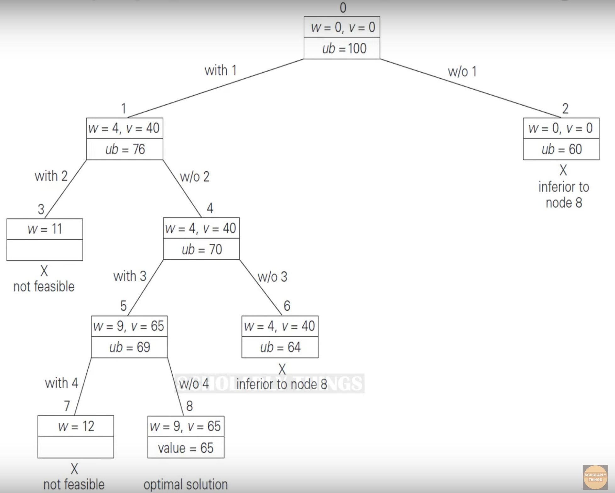
The problem is solved using branch-and-bound algorithm described in this video. It uses a binary tree where the left branch refers to the combination when an item is included while the right one is when it’s excluded. At every step, the algorithm looks for the highest upper bound:

\[ub = v + (W-w)\frac{v_B}{w_B},\]

where $v$ is the value of the total selected items, $W-w$ the remaining weight and $\frac{v_B}{w_B}$ refers to the best payoff among the items that are not yet included.

A brute-force approach would have required to go over $2^4=16$ combinations whereas here we go over 9 combinations only. This is because we leveraged on the value to weight ratio.