Neural network

Those notes are largely inspired by the tutorials of Andrew Ng.

While counting the layers, we usually don’t include the input layer. The first schema (left) is a 1-layer neural network whereas the second schema (right) is a 2-layers neural network. We notice that a 1-layer neural network doesn’t have any hidden layer.

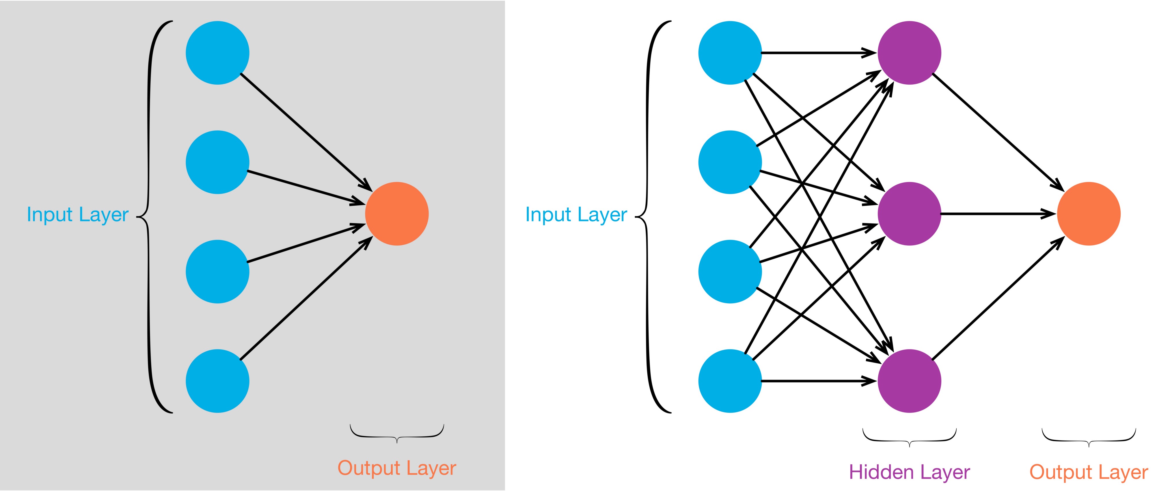
1-layer neural network

A 1-layer neural network can be seen as a logistic regression. The below explanation is largely inspired by the example from coursera (deeplearning.ai)

Let us take the example of an image that we want to classify in a binary way: man/woman

The picture is vectorized as a vector of pixels : \(\begin{pmatrix}x_1 \\ \vdots \\ x_p \end{pmatrix}\)

We use a regression to predict if it’s a man/woman:

$y=\omega^Tx + b$

Note: $x$ are all the pixels of one image.

We want a probability in output (if it’s $\ge 0.5$ then we say it’s a man).

We thus want the output to be $\widehat{y}=\sigma(\omega^Tx + b)=\mathbb{P}(y|x) \in [0,1]$

(see regression part to get more details on the sigmoid)

Now since it’s a binary classification, we want the $y$ (real value) to be $0$ or $1$.

Thus, the loss function is:

We notice that the loss function decreases when $y \neq \widehat y$.

The cost function is the empiric loss on all examples:

Forward propagation

• First arrow: regression

• Second arrow: probability

• Third arrow: error

Backward propagation

The idea is: with the error computed on the last step, we go backward in order to correct the parameters $\omega$ and $b$.

To find the new value of $\omega$ we look for its change ($d \omega$) that we can obtain thanks to the Chain rule. It consists of decomposing the derivative into successive ones.

The parameters that are udpated during the training are the weights $\omega$ and the bias $b$. Thus we need to compute $\frac{d\mathcal{L}}{d\omega}=”d\omega”$ and $\frac{d\mathcal{L}}{db}=”db”$ .

First the weights:

Then the bias:

Note: we can see that the updated weight depends on the previous prevision $a$. This is why it is necessary to recompute the predicted value at each iteration.

for i in range(num_iterations):
            
    # Cost and gradient calculation
    grads, cost = propagate(w, b, X_train, Y_train) # propagation on ALL the training sample
            
    # Retrieve derivatives from grads
    dw = grads["dw"]
    db = grads["db"]
            
    # update parameters
    w = w - learning_rate * dw
    b = b - learning_rate * db
            
    # Record the costs
    costs.append(cost)

def propagate(w, b, X, Y):
        
    m = X.shape[1]
       
    # FORWARD PROPAGATION (FROM X TO COST)
    A = sigmoid(np.dot(w.T,X)+b)
    cost = (- 1 / m) * np.sum(Y * np.log(A) + (1 - Y) * (np.log(1 - A))
        
    # BACKWARD PROPAGATION (TO FIND GRAD)
    dw = (1/m)*np.dot(X,(A-Y).T)
    db = (1/m)*np.sum(A-Y)

2-layer neural network

Forward propagation

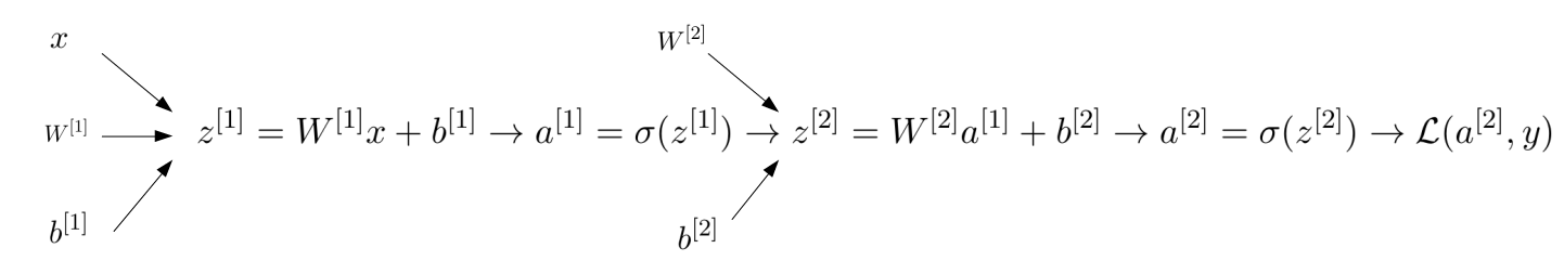
The main difference with the case of 1 layer is that now there are two sets of weights and biases. Moreover, the first set of weights is not a 1-column vector but a matrix.

Backward propagation

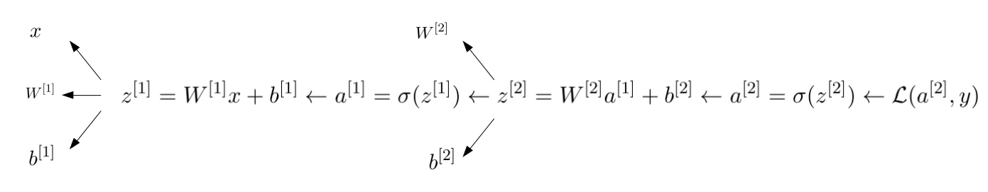
We now need to update 4 parameters: $W^{[1]}, b^{[2]}, W^{[2]}, b^{[2]}$.

For $W^{[2]}$:

For $b^{[2]}$:

For $W^{[1]}$:

Warning: the element-wise product is necessary to have the right dimensions at the end.

For $b^{[1]}$: