Framework

LDA is an unsupervised method mostly used for topic modelling in NLP. It is part of the generative models because the goal is to learn an underlying distribution by estimating the parameters. Here the parameters are $\theta$ and $\varphi$ (i.e. distributions) which can be deduced from the posterior distribution $\mathbb{P}(z | w)$ computed through the Gibbs sampling method as explained below.

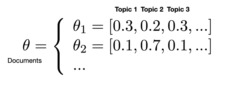
The basic idea of LDA is that each document is represented as a distribution over topics and each topic as a distribution over words.

The representation of documents as distribution over topics is called “random mixture over latent topics” because:

• the topics are drawn from a random distribution (Dirichlet)

• the topics are not known (latent) and need to be learned

We have $\theta \sim Dir(\alpha)$ and $\varphi \sim Dir(\beta)$.

Dirichlet distribution

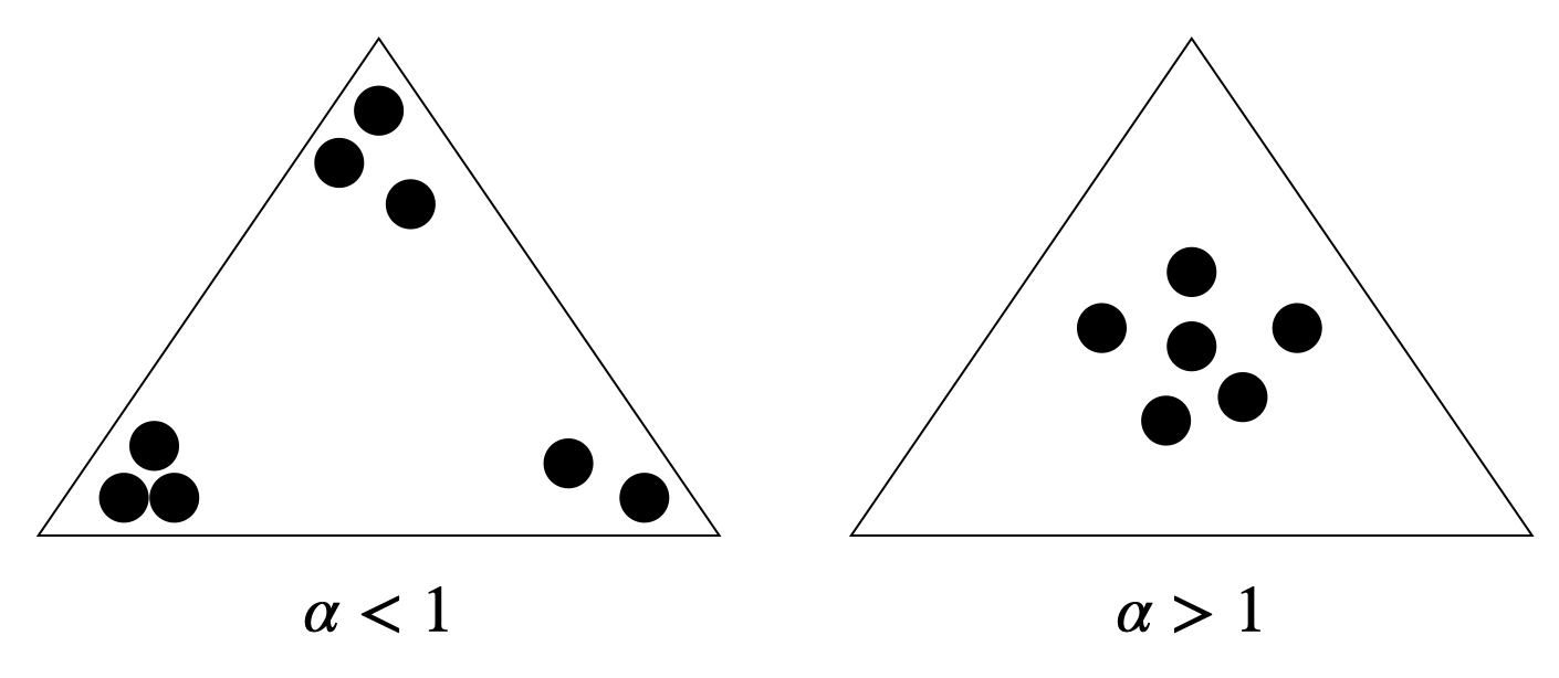
The Dirichlet distribution is a multivariate distribution (the random variable is a vector). It’s a generalization of the beta distribution and also the conjugate of the multinomial distribution. The parameter represents the prior distribution of the observations. It is common to choose low $\alpha$ and $\beta$ since documents are likely to be related to few topics only and topics related to few words only. We can represent the distributions with a triangle:

Problem formulation

We want to infer the posterior distribution of the latent variables (documents & topics). In other words, we want to determine the distribution of topics for each document:

\[\mathbb{P}(\theta, z | w, \alpha, \beta) = \frac{\mathbb{P}(\theta, z, w| \alpha, \beta)}{\mathbb{P}(w | \alpha, \beta)}\]

The denominator is the marginal probability of a document (= probability of generating a word). However, this quantity is intractable i.e. very hard to compute in a reasonable amount of time due to the large amount of parameters.

Gibbs sampling

To approximate the above quantity we can use approximate inference algorithms. Among them, the Markov Chain Monte Carlo (MCMC) consists in generating a vector $x_t$ only based on $x_{t-1}$. In the case of LDA, for each document we compute the below quantity:

\[\mathbb{P}(z_i | z_{-i}, d, w, \alpha, \beta) \propto \mathbb{P}(w | z_i, z_{-i}, \beta)\mathbb{P}(z_i | z_{-i}, d, \alpha)\]

Intuitively, we want to attribute a topic to a word assuming that every topic/word is correctly classified (i.e. based on the previous state represented by $z_{-i}$). For clarity purposes we can simplify the above equation and find again the Bayes formula:

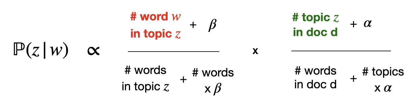
\[\mathbb{P}(z | w) \propto \mathbb{P}(w | z)\mathbb{P}(z)~~~~~~(E)\]

Numerically:

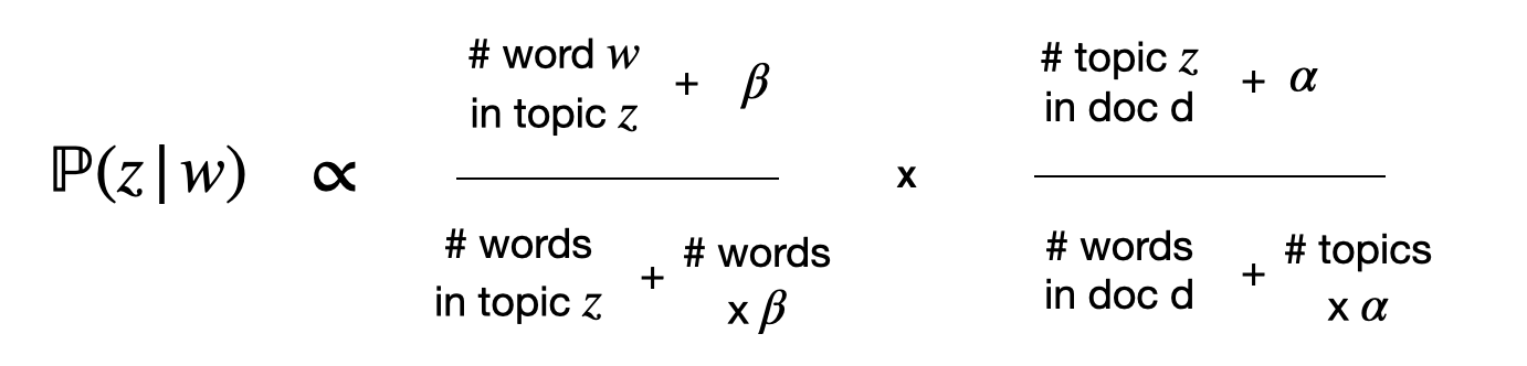
Note: the summed elements like $+ \alpha$ are here since we don’t want probabilities for words/topics that are not here to be zero, otherwise they will set the whole product to be zero. See additive smoothing.

Implementation

An implementation of the method can be found here. In this implementation, the document and the word are not drawn from any distribution; since it’s a simplified example, we simply loop across all documents and words. Below is the pseudo code:

Non-technical explanation: for each document, for each word, we map it to the best topic assuming the other words/topics are correctly mapped.

Explanations on why it works

The algorithm relies on 2 main properties:

1- Articles are as monochromatic as possible i.e. each articles should be associated with few topics only.

2- Words are as monochromatic as possible i.e. each word should be associated with few topics only.

In a nutshell, the algorithm accentuates those properties throughout its run. The excel screenshot below shows that we need only 2 iterations so that we get the right distributions of topics for each articles (last upper column).

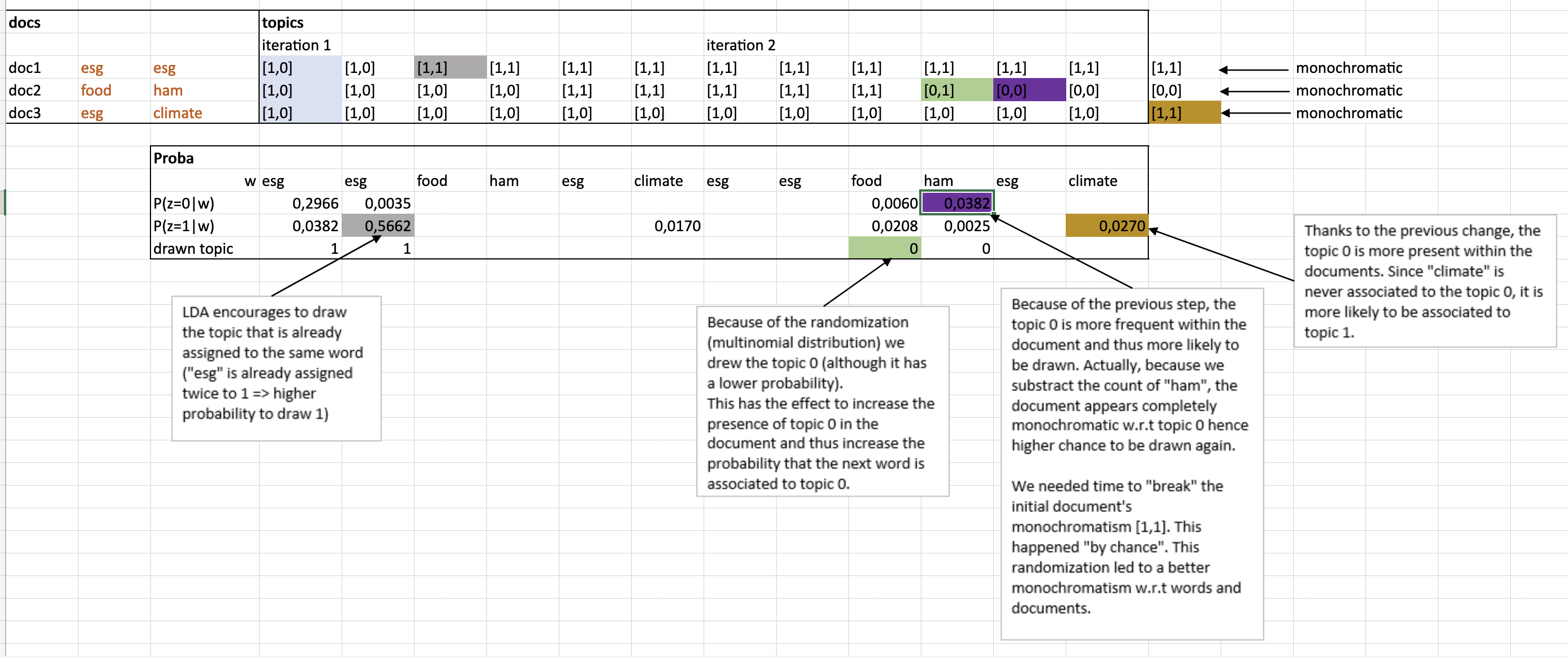
At the beginning, every word is randomly mapped to a topic. When a word is often mentioned, it thus has a high count w.r.t to one topic. The more a word is associated to a topic, the more likely it is to be again associated to the same topic in the future (= accentuation of monochromatism 2). See example of grey cell (“esg”) in the excel screenshot. This behaviour is reflected in the red quantity.

The randomization allows to test word-topic combinations. If a new combination leads to more monochromatism, it will be accentuated in the future (= accentuation of monochromatism 1). See example of green and violet cells in the excel screenshot. This behaviour is reflected in the green quantity.

Official algorithm

1. Choose $\theta \sim Dir(\alpha)$. Recall that $\alpha$ is the prior probability distribution. When using $\alpha < 1$ we ensure that there are just few topics for each document (monochromatic documents).

2. For each word:

   (a) Choose a topic $z \sim Multi(\theta)$. Based on the document, we can choose a topic based on the distribution of topics for the document.

   (b) Compute $\mathbb{P}(w | z, \beta)$. We find the best word to be associated to the topic we drew at the previous step.