Hierarchical clustering contains two types of methods:

• Agglomerative: bottom-up approach (from leaves to root)

• Divisive: top-to-bottom (from root to leaves)

Agglomerative clustering

Agglomerative clustering is a sequential process:

• First, all data points are considered as separate clusters.

• Then, step by step, clusters that are closed to each other merge.

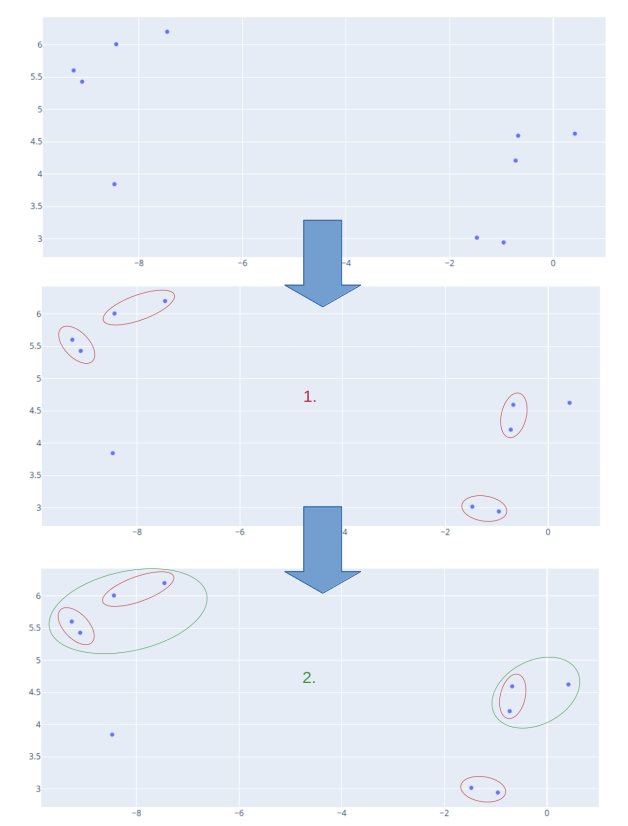
The first two steps of an example are displayed below:

The whole merging process can be vizualized using a dendrogram where the y-axis is the distance between two points/clusters. In x-axis we see the data point index.

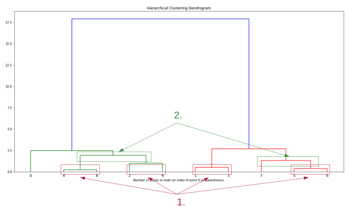
Note: In case of a large sample, it is possible to display only the last steps of the algorithms (see level parameter in scipy)

There are three main parameters to choose:

• Distance metric: this is the metric used to compute the distance between two data points.

• Distance function / rules: this is the function used to compute distance between two clusters. It’s a function of the distance metric.

• Number of clusters

Distance functions

The most common distance functions are:

Minimum distance (also called single-linkage-clustering):

\[D(A,B) = min\{d(x,y): x \in A, y \in B\}\]

Average distance:

\[D(A,B) = \frac{1}{|A| |B|} \sum_{x \in A,~y \in B}d(x,y)\]

Max distance (also called complete-linkage-clustering):

\[D(A,B) = max\{d(x,y): x \in A, y \in B\}\]

Number of clusters

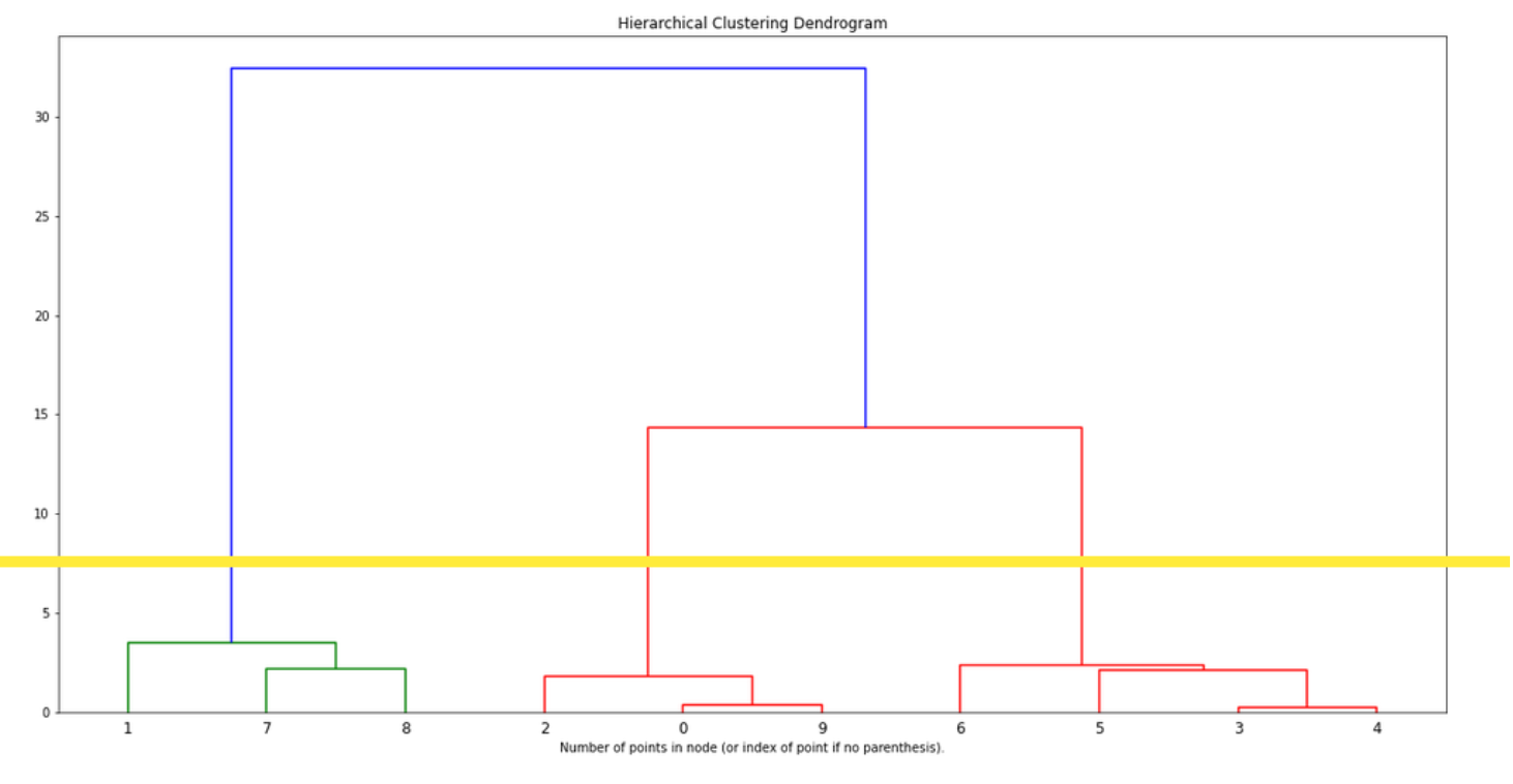
To select the number of clusters, we can look at the dendrogram: we focus on groups that are linked by long lines. Since the lines represent the distance between data points or clusters, a group of clusters that are far away from each other will be linked with long lines.

In the below dendogram, it’s quite clear that 3 clusters are well separated:

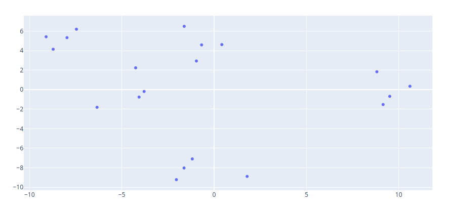
On the below example (with associated dataset), we could select 3 or 5 clusters.