Gradient Boosting

Gradient Boosting Method is an agorithm that is part of ensemble methods.

There are many different implementation of this algorithm; the below one (src: StatQuest) is one of the most generic and understandable.

Initialize model with constant value
for $m = 1$ to $M$:

Output $F_M$

Step 1: initialize model with constant value

\[F_0 = \underset{\hat y}{argmin} ~\Sigma_{i=1}^n \mathcal{L}(y_i,\hat y)\]

We note that $\hat y$ is constant and doesn’t depend on $i$. Consequently, optimizing this equation using MSE will lead to $\hat y = \bar y$:

Note: $MSE := \frac{1}{n}\Sigma_{i=1}^n (y_i - \hat y)^2$ thus to use MSE in our case we need to have $\mathcal{L}: (y,\hat y) \to (y-\hat y)^2$ but we usually choose $\mathcal{L}: (y,\hat y) \to \frac{1}{2}(y-\hat y)^2$

$\frac{\partial MSE}{\partial \hat y} = 0$

=> $\frac{2}{n}(y_1 - \hat y) + … + \frac{2}{n}(y_n - \hat y) = 0$

=> $\hat y = \Sigma_{i=1}^n \frac{y_i}{n} = \bar y$

Step 2: loop on the number of estimators

(A) Pseudo-residuals

\[r_{im} = - \frac{\partial \mathcal{L}(y_i, F(x_i))}{\partial F(x_i)} \text{ for } i=1,...,n\]

The gradient of the loss function is $\frac{\partial \mathcal{L}}{\partial \hat y} = -(y - \hat y)$

Residuals as seen in linear regression are typically written as such: $res = y - \hat y$. Thus, gradient boosting uses negative residuals, also called pseudo-residuals.

Note 1: pseudo-residuals are just the derivatives of the loss function; that’s why we call it gradient boosting.

Note 2: $F(x_i)$ is equivalent to writing $\hat y$. It’s the prediction of each record.

Reminder: the prediction of a decison tree is found in navigating from the root to the leaf where the sample is classified.

(B) Fit a weak learner with $r_m$ as target values

h = tree.fit(x, res)

Weak learners (see definition in Adaboost section used in gradient boosting are typically decision trees. These learners are trained on residuals.

Thus, this step consists in building a small tree.

(C) Compute a unique output for each leaf

We could call this step: “harmonization of predicted values”.

For $j=1,…,J_m$:

\[\gamma_{jm} = \underset{\gamma}{argmin}~\Sigma_{x_i \in R_{ij}} \mathcal{L}(y_i, F_{m-1}(x_i)+\gamma)\]

The loop “For $j=1,…,J_m$” means we iterate on all leafs of the previously built tree.

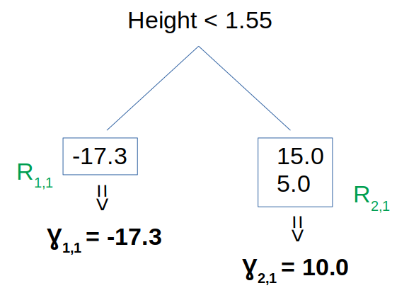
This step consists in building a unique output for each of its leaf. $R_{j,m}$ are the terminal regions, that is, the leafs of the tree.

In the below picture the first weak learner is shown. Here $J_m=2$ since there are 2 leafs only.

We also consider the MSE as a loss function, so $\gamma_{jm}$ is equal to the averages of the leaf outputs.

(D) Update the function

\[F_m(x) = F_ {m-1}(x) + \alpha \Sigma_{j=1}^{J_m} \gamma_{jm} \unicode{x1D7D9}(x \in R_{jm})\]

$\alpha$ is the learning rate used to reduce overfitting.

The summation is here only in case one record $x$ ends up in several leafs.

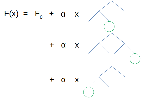
Step 3: Output the function

$F$ is the output of the algorithm and is just a combination of several trees. To find the predicted value of a record, we would need to sum all predicted values of each tree (weighted by the learning rate $\alpha$). Below is an illustration of the computation of the final prediction for a record $x$: