The use of SHAP values is a simple method to measure the impact of features on any model. Intuitively, it consists in adding/removing a feature and measure the impact of the removal on the prediction. Thus, it aims at finding marginal contributions of features.
The concept of SHAP is based on Lloyd Shapley’s results on game theory. Shapley’s main idea is that members should receive payments proportional to their marginal contributions to the society.
Note: the explanation of the game theory part is based on Stanford tutorial.
The main question is: what weighting system should we use?
Let $N$ be a coalition with all members involved, and $S$ a coalition with any member(s).
$v$ is the value brought to the society by a specific coalition.
Shapley considers several axioms:
Symmetry: for all $S$ that contains neither $i$ nor $j$, $i$ and $j$ are interchangeable if $v(S \cup {i})=v(S \cup {j})$. Then interchangeable agents should receive the same payments: $\phi_i(N,v)=\phi_j(N,v)$.
Intuitively, agents who contribute the same should receive the same payments.
Dummy players: $i$ is a dummy player if the amount that $i$ contributes to any coalition is $0$: for all $S$, $v(S \cup {i})=v(S)$. Then for any $v$, if $i$ is a dummy player: $\phi_i(N,v)=0$.
Intuitively, dummy players should receive nothing.
Additivity: if we can separate a game in two parts: $v=v_1 + v_2$, then we should be able to decompose the payments: $\phi_i(N, v_1+v_2) = \phi_i(N, v_1) + \phi_i(N, v_2)$.
For instance, we can consider a game that consists in producing fruits during two days. An agent will receive equally the fruits production of day 1 and day 2 than receiving the total production for these two days.
Based on the previous axioms, it turns out that there is only one way of defining the payment of each agent:
\[\phi_i(N, v) = \frac{1}{|N|!} \Sigma_{S \subseteq N\setminus \{i\}} |S|! (|N| - |S| - 1)! (v({S \cup \{i\}}) - v(S))\]Warning: here $|.|$ is the cardinality of a set (not the absolute value function!)
$v({S \cup {i}}) - v(S)$ is the marginal contribution of agent $i$.
The rest of the formula consists in weighting the marginal contribution with all possible coalitions. More specifically:
$|S|!$ is the number of times $S$ could have been formed.
$(|N| - |S| - 1)!$ is the number of times the remaining agents could have been added.
$\frac{1}{|N|!}$ is used to average across all different possible coalitions.
Application to machine learning - visual approach
The next part of this section is inspired by a very good tutorial on how the Shapley value is applied to machine learning.
Here, the “game” is what produces the outcome of a model. The “agents” or “players” are the features of the model.
Let’s consider a model that consists in predicting the income of an individual based on the age, the gender and the job.
To define all the possible coalitions, we use the mathematical concept power set:

Once the training is done, we compute the prediction for each coalition:
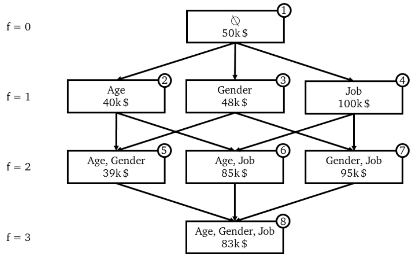
We note that an edge (or an arrow) is the effect of a marginal contribution.
With machine learning notation, the marginal contribution is:
\[MC_{feat 1, \{feat 1, feat 2\}} = Predict_{feat 1, feat 2}(X) - Predict_{feat 2}(X)\]Note: for classification problems that output probabilities, the marginal contribution is the difference in probabilities for each class. The final output of SHAP is split by classes:.

$MC_{feat 1, \{feat 1, feat 2\}}$ should be read: “the effect of feature 1 in coalition {feat 1, feat 2}”.
In the above example, $MC_{Age, \{Age\}} (X) = 40k - 50k = -10k$.
The SHAP value is defined as such:
\[\begin{align*} SHAP_{Age}(X) &= \omega_1 MC_{Age, \{Age\}}(X) \\ &= + \omega_2 MC_{Age, \{Age, Gender\}}(X) \\ &= + \omega_3 MC_{Age, \{Age, Job\}}(X) \\ &= + \omega_4 MC_{Age, \{Age, Gender, Job\}}(X) \end{align*}\]Under the constraint: $\omega_1 + \omega_2 + \omega_3 + \omega_4 = 1$
Thus, the SHAP value is the average of all impacts a feature brings to every coalition.
But how to find the weights?
The weights are based on the number of edges for the specific level of the power set we are looking at. Mathematically, it’s the inverse of the function $f*C_{f}^F$.
For example, for the level $f=2$, $\omega_3 = \frac{1}{2*C_{2}^3} = \frac{1}{6}$.
Warning: if feature 1 contributes more than feature 2, it doesn’t mean that feature 1 improves more the model than feature 2! As mentioned by the author, “SHAP values of a model’s output explain how features impact the output of the model, not if that impact is good or bad”.
One of the main limits of SHAP is that it has a lot to compute. The cardinality of a power set is $2^n$. This is thus the number of model to train (with the same parameters and input data) to compute the Shapley value ($n$ = number of features = $F$ in our case). Fortunately, the method used approximation without computing all possible cases.
Application to machine learning - SHAP package approach
The following explanation is based on the research paper behind the SHAP package.
The SHAP package bases its results on the following definition.
An additive feature attribution method is a linear function of binary variables:
\[g(z') = \phi_0 + \sum_{i=1}^M \phi_i z_i'\]Where $z’ \in \{0,1\}^M, M$ is the number of simplified input features, and $\phi_i \in \mathbb{R}$ are the Shapley values. $g$ is the explanation model and $z’$ is the vector representing which feature to include ($1$) or not ($0$).
The SHAP package also bases its results on additional properties similar to the ones mentioned in the introduction (theoretical part).
To find $\phi_i$ (Shapley values), we use the same approach as LIME i.e. to minimize $L(f,g,\pi)$ where $f$ is our original function. It turns out that the only solution to this problem is:
\[\pi(z') = \frac{M-1}{C_{|z'|}^M |z'|(M-|z'|)}\] \[L(f,g,\pi_{x'}) = \sum_{z' \in Z}[f(h_x(z'))-g(z')]^2 \pi(z')\]The proof is in the supplementary material of the article.
The weight function consists in penalizing mixed combinations (e.g. $[0,0,1,1]$) and encouraging more “pure” combinations (e.g. $[0,1,1,1]$). The intuition behind such behaviour is explained on Christoph Molnar’s website:
“We learn most about individual features if we can study their effects in isolation. If a coalition consists of a single feature, we can learn about this feature’s isolated main effect on the prediction. If a coalition consists of all but one feature, we can learn about this feature’s total effect (main effect plus feature interactions). If a coalition consists of half the features, we learn little about an individual feature’s contribution, as there are many possible coalitions with half of the features.”
The loss function shows us that the problem can be solved just like a weighted linear regression. The estimated coefficients are the Shapley values themselves!
Reminder: the weighted linear regression has the form $argmin||X\theta - Y||^2W$. In our case, $X$ is the vector of all possible coalitions and $Y$ the prediction results for each combination. The solution to this problem is $\theta = (X^TWX)^{-1}X^TWY$.
Note: the classical assumptions in linear regression (e.g. homoscedasticity, exogeneity) may be violated. However I believe the model can’t be improved: the set of features represents all the possible combinations (= population) and thus can’t be changed. In other words, in the Shap framework the number of features is fixed. An interesting article on the limits of Shapley values with geometrical representation.
See this repo for more details on its implementation (application to rule-based models).