We want to approximate $f: \mathcal{X} \to \mathcal{Y}$, $\mathcal{X} \in \mathbb{R}^p$, $\mathcal{Y}={1,…,L}$

We note:

$x=(x_1,…,x_p)^T \in \mathcal{X}$ a sample

The distance between 2 samples: $d: \mathbb{R}^p \times \mathbb{R}^p \to \mathbb{R}$

$\mathcal{D}_n={(x_i,y_i),i=1,…,n}$ the training set with $n$ samples and labels.

For each new sample $x \in \mathbb{R}^p$, we determine the set of k nearest neighbors among all the train set.

Note: a sample is an observation, that is $x^T=(x_i^{(1)},…,x_i^{(p)})$. We thus compute the distances between vectors of dimension $p$.

The most basic distance metric is the Euclidean norm: $d(u,v)=||u-v||^2=\Sigma_{i=1}^p(u_i-v_i)^2$

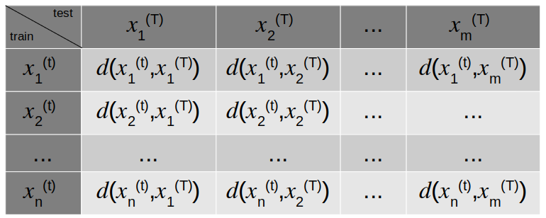
The algorithm consists in building a distance matrix with the test sample in columns (power $(t)$) and the train sample in rows (power $(T)$) as shown below:

Note: in this matrix, the training sample is of size $n$ and the test sample is of size $m$.

We then sort the matrix column-wise in ascending order in order to find train data points with smallest distance to the test data point.

For each test data point, we keep the $k$ smallest distances (i.e. the $k$ first rows of the sorted matrix) and we look at their labels. The Python function argsort() allows us to keep indices when sorting. We define the rank of a neighbor as:

\(r_k(x)=i^* \text{ if and only if:}\) \(d(x_{i^*},x)=\underset{1 \le i \le n \\ i \neq r_{1},...,r_{k-1}}{\operatorname{min}}d(x_i,x)\)

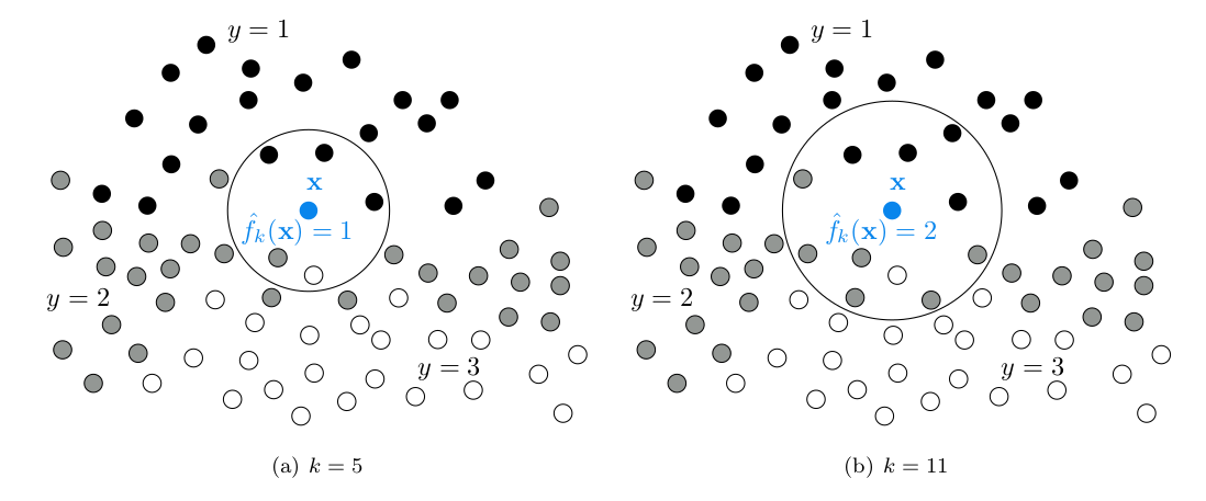
The most basic rule is to take the most frequent label among the $k$ neighbors. In the below schema we consider $k=5$ and $k=11$ with three classes ($L=3$) that are drawn respectively in black ($y=1$), grey ($y=2$) and white ($y=3$).

Note: the fit() function of the KNNClassifier is just an affectation of the training data to the object; the distance computation is done in the predict().

The biggest advantages of the KNN algorithm are:

• It’s a simple and intuitive algorithm that can be easily explained and understood.

• Its parameter can be easily optimize e.g. using cross validation.

The biggest drawbacks are:

• The prediction can be computationally expensive because we need to compute all distances between test and train data.

• It has a high variance: the prediction can be strongly different if the data are slightly different.

Alternative

This alternative doesn’t change the knn selection, it only changes the class attribution in the neighborhood. It gives more weights to very small distances. The higher $h$, the higher we favor small distances ($exp$ function becomes steeper).

class KNNClassifier(BaseEstimator, ClassifierMixin):
    """ Homemade kNN classifier class """
    def __init__(self, n_neighbors=1):
        self.n_neighbors = n_neighbors
    
    # the training step only consists in storing training data
    def fit(self, X, y): 
        self.X = X
        self.Y = y
        return self
    
    def predict(self, X):
        n = len(self.X) # size of train set
        m = len(X) # size of test set
        dist_mat = []
        for i in range(n): # we loop on every element of the train set
            dist_vect = []
            for j in range(m): # we loop on every element of the test set
                dist_vect.append(euclidean_distance(self.X[i], X[j]))
            dist_mat.append(dist_vect) 
	  # len(dist_vect) = m (nb of features; all the distances for one observation)
            
        dist_mat = np.asarray(dist_mat) 
        # dist_mat.shape = (n,m); T_test in column, X_train in row
        
        # dist_mat = metrics.pairwise.pairwise_distances(
				X, Y=self.X, metric='euclidean', n_jobs=1
				)
            
        idx_sort = np.argsort(dist_mat, kind='mergesort', axis=0)  
        # idx_sort.shape = (n,m); dist_mat sort column-wise
        # mergesort is a stable way to handle equal numbers: 
        # if equal, the order of indices in the output is the same as in the input
        
        idx_sort_knn = idx_sort[:self.n_neighbors,:] # resize with the number of knn
        return getBestClassFromCount(idx_sort_knn, self.Y)